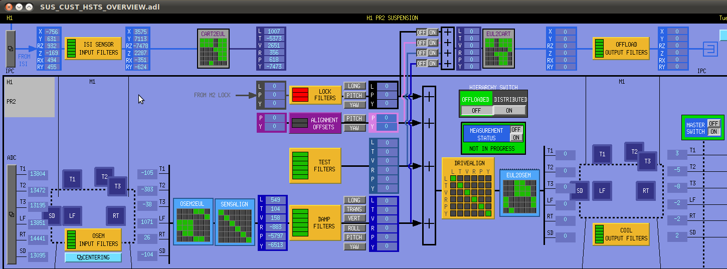
I've completed the installation of the H2 SUS PR2 ISI WIT and OFFLOAD path, such that the H1 HAM3-ISI GS13s are now projected into the H2 SUS PR2 Suspension point basis, and the H2 SUS PR2 M1 offload signal may be sent to the HAM3-ISI. Details of the design are discussed below. The following channels are now calibrated into (nano)meters or (nano)radians of motion at the H1 HAM3-ISI center of actuation and at the H1 SUS PR2 suspension point, respectively:

H1:SUS-PR2_M1_ISIINF_${CARTDOF}_OUT_DQ 
H1:SUS-PR2_M1_ISIWIT_${EULERDOF}_DQ

which are stored in the frames at 1024 Hz, where ${CARTDOF} = [X, Y, RZ, Z, RX, RY] and ${EULERDOF} = [L, T, V, R, P, Y].

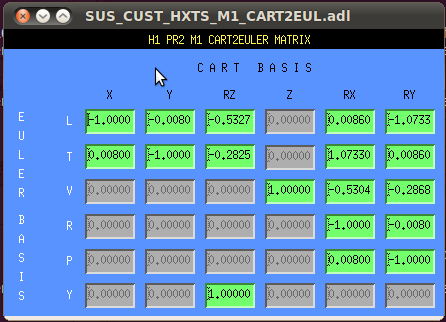
I attach a couple of screenshots of the implementation in MEDM. The paths are shown at the top of the HSTS overview screen (shown in H1SUSPR2_SEISUSPaths_OverviewScreenShot.png). Clicking inside the ISIINF bank (shown in H1SUSPR2_SEISUSPaths_ISIINF.png), one sees the 4k to 16k AI filter in FM1, the conversion from ideal inertial sensor response to displacement lies in FM5, and additional gain-only filters have been installed into FMs 9 and 10, if the user so chooses to convert the displacement signal either from nanometers (nanoradians) to micrometers (microradians) in FM9 or from nanometers (nanoradians) to meters (radians) in FM10. Finally, I show the CART2EUL matrix for H1 SUS PR2 (see H1SUSPR2_SEISUSPaths_CART2EULMatrix.png), taken from
/opt/rtcds/userapps/release/isc/common/projections/ISI2SUS_projection_file.mat
computed as described in T1100617, and installed with
/ligo/svncommon/SeiSVN/seismic/Common/MatlabTools/fill_matrix_values.m

I also attach three sets of plots explaining the design:
isiinf_tonmdesign_2012-10-30.pdf --
Here, I elucidate the thought process behind the design of the "to_nm" filter in FM5 of the ISIINF filter bank, breaking the filter down into its various parts / functions.
- The GS13 signals, in the ISI's center-of-actuation, Cartesian basis (picked off from the input to the blend filters) arrives calibrated into an ideal inertial sensor response, which asymptotes to 1 [nm/s] at high-frequency (above ~1 [Hz]), and rolls off at low frequency as f^2. 
- The first step is to invert this response, shown by the "1 Hz Ideal Inertial Sensor Response to Velocity" in BLUE, leaving the signal in [nm/s] velocity units at all frequencies. This portion of the filter (in Matlab notation) is
velcal = zpk(-2*pi*[pair(1,45)],-2*pi*[0,0],1)
- Next, the signal is integrated once (i.e. the GREEN filter; convdisp = zpk([],-2*pi*[0],1)), to convert to [nm] displacement units, resulting in the CYAN filter,
velcal*convdisp = zpk(-2*pi*[pair(1,45)],-2*pi*[0,0,0],1)
Note: this is the filter that one typically uses to "finish" the calibration of the inertial sensor offline to compute an ASD of the signal.
- Finally, because we still want to have a usable time series and not have a calibration filter with infinite step response, we roll off the calibration such that signal is low-passed/AC-coupled at 10 mHz, with the (RED) filter portion, rolloff = zpk(-2*pi*[0,0,0,0],-2*pi*[0.01,0.01,0.01,0.01],1) resulting in the final, MAGENTA, TOTAL filter,

velcal * convdisp * rolloff = zpk(-2*pi*[0,0,0,0,pair(1,45)],-2*pi*[0,0,0,0.01,0.01,0.01,0.01],1)
                            = zpk(-2*pi*[0,pair(1,45)],-2*pi*[0.01,0.01,0.01,0.01],1)

which rises as f from DC, turns over at 10 mHz, falls as 1/f^3, crosses unity at 1/(2*pi*1), knees at 1 Hz to fall as 1/f out to high frequency, as expected. The corner frequency of 10 mHz was chosen for several reasons:
(1) It's roughly equivalent to the corner frequency of the T240s on ST1 of the BSC-ISI
(2) The GS-13 signals at these frequencies are dominated by sensor-noise.
(3) We wanted to still accurately reproduce the magnitude/amplitude of the signal at the microseism.
(4) We wanted the time series to be manageable during normal operation.

BE AWARE Though the magnitude/amplitude of the signals calibrated in this fashion are accurately reproduced down to ~50 [mHz], the phase lags the real signal by the difference between MAGENTA and CYAN, which already lags 22.73 [deg] by 0.1 [Hz] and as much as 180 [deg] by 10 [mHz]. (Several different options were tossed about that would have potentially improved the phase reproduction (elliptic filters, butterworth filters, etc.) but we figured, for now, perfect is the enemy of good enough.)

isiinf_filters_2012-10-30.pdf --
pgs 1-2 show the magnitude and phase of the as-implemented AA/AI filter (used as a 4k to 16k AI filter in the ISIINF banks to receive the GS13 signals, and as a 16k to 4k AA filter in the OFFLOAD banks to send the SUS offload signals out to the ISI). The filter's bump maxes out at 2.11 dB above unity around 1350 Hz, and has -79.38 dB isolation the 4096 Hz notch. The filter was implemented using the ZPK portion of the foton design suite, with 

               Mag   Phase       Mag    Phase
poles  = [pair(2*850, 55  ) pair(2*1048, 70  )];
zeros  = [pair( 4096, 89.9) pair(2*4096, 89.9)];


The details of the design for the AA/AI filter can be found in the old SEI Log entry 1937. This filter was designed to have better phase loss and anti-imaging properties at f < 100 Hz than the "standard" CDS 4k AA/AI filter, with only 5.5 deg lost at 100 Hz (the standard has ~10 deg loss). Since Lantz determined this was better for what seismic typically does with these signals -- and it's what they use to up/down-sample their signals from the IOP -- I figured "why be different?" Lantz approves.

pg 3-4 shows the magnitude and phase of the as-implemented "to_nm" filter, equivalent to velcal * convdisp * rolloff from above, but the design string in foton is subtly different because of Sigg's vs. Matlab's convention choices:

    zeros                           poles                 gain
zpk([0;0.707+i*0.707;0.707-i*0.707];[0.01;0.01;0.01;0.01],1.59e7,"n")

(note the gain of 1.59e7 = 1/(2*pi*(0.01)^4) to normalize the rolloff properly in foton's convention.)

isiinf_H1SUSPR2_2012-10-30.pdf --
These plots show the ASD and Magnitude, Phase, and Coherence of the Transfer Function between exemplary channels:
H1:ISI-HAM3_BLND_GS13X_IN1_DQ -- the inputs to the blend filters, fresh off of the ISI, calibrated in [nm/s] "offline" using DTT's calibrator with a filter identical to velcal above (scaled into [m/s] by a factor of 1e-9), and then displayed in (integrated to) displacement courtesy of DTT (which is identical to convdisp above). 
H1:SUS-PR2_ISIINF_X_OUT_DQ -- the output of the ISIINF, after AI filtering and calibrated "online" to [nm] (and then scaled to [m] by 1e-9 in DTT).
H1:SUS-PR2_ISIWIT_L_DQ -- the final result of interest: the GS13s calibrated "online" and propogated through the CART2EUL matrix to the H1 SUS PR2 suspension point.
This data was taken with the ISI active control loops completely OFF (no damping, no isolation, no nothing).

Here, we see lots of fun things:
(ASD) 
(a) Above the 10 mHz rolloff, once calibrated into the same units, the X signal is identical between the input to the blends (RED) in HAM-ISI land and the output of the ISIINFs (BLUE) in SUS land. Below the roll-off, the signals begin to diverge at ~50 mHz as expected. 
(b) The point of this whole shebang: The signal projected to the susp. point (GREEN) is different from simply assuming the X motion (BLUE) is what's input. Here, in L, we see significant contribution from both X and RY, most notably at the ~1 Hz RY resonance (a factor of two with the resonance undamped). I'm very interested to see what other degrees of freedom look like, and under different conditions of the ISI...

(COH) 
(a) As expected the coherence between the signal in ISI land and the signal in SUS land drops, simply because of the roll off filter.
(b) The coherence drops along the various cross-couplings between ISI Cartesian, center-of-actuation, basis and SUS Euler, suspension point, basis. 

(TF) 
(mag) This basically just reproduces the product of the calibration and AI filters in the bank as expected, but there are some interesting features where the cross-coupling is going on 
(pha) Same as mag. Note that L is 180 deg out of phase with X because -- you guessed it -- PR2 is pointed in the -X direction.

In conclusion:
This well-defined, in-the-same-basis, peaches-to-peaches, signal opens up a whole bunch of new possibilities for modeling the suspension's motion, least of all, for starters, it should certainly require a lot less (i.e. no) offline post processing for modelers, commissioners, and glitch hunters alike.

Now that I've got the first-article filters in place, I've already got the SEI/SUS basis matrices (for every SUS that has a system's drawing), it should be very straight-forward to get the rest of the SUS up to speed. 

Stay tuned for new found understandings!