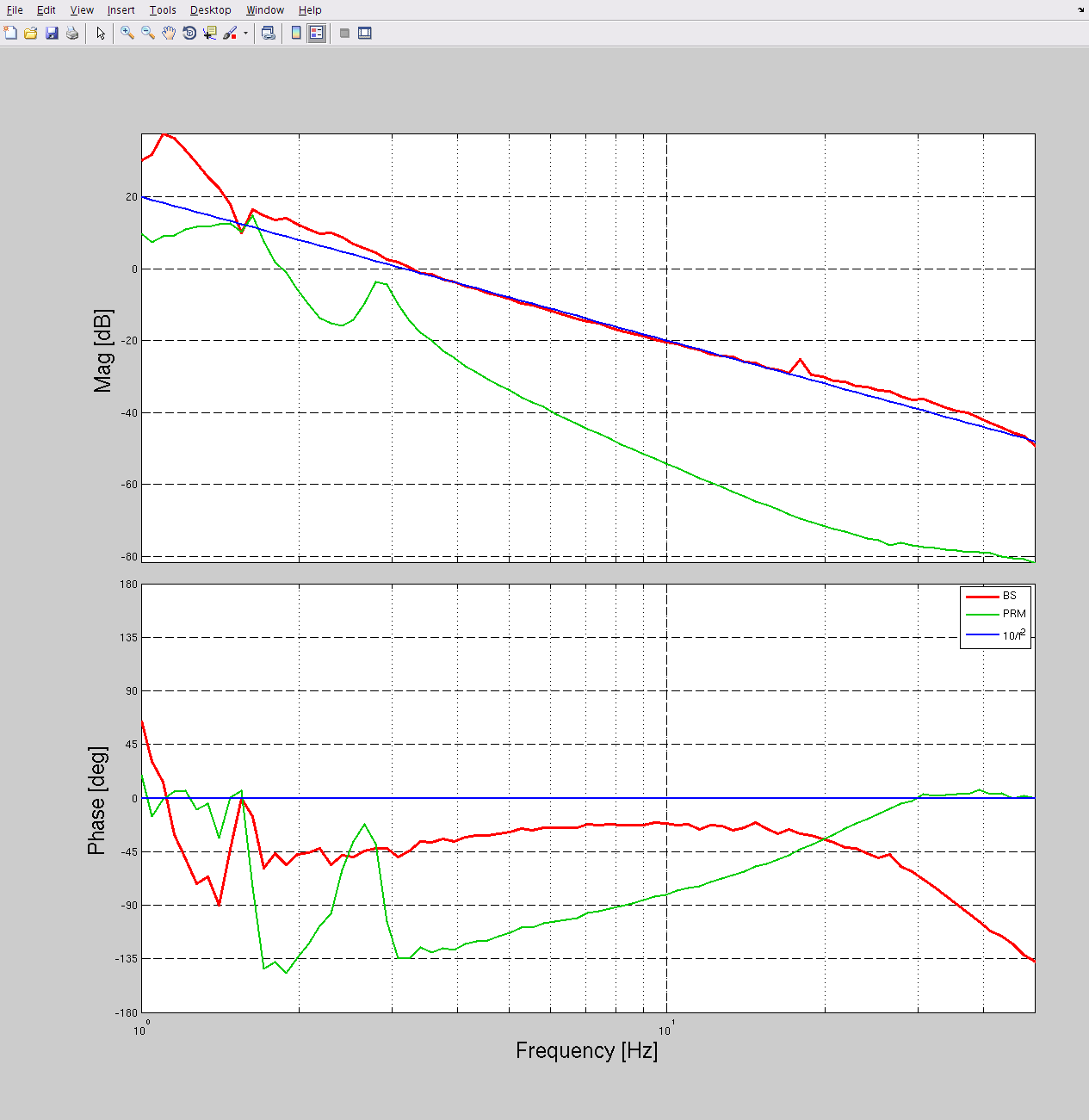
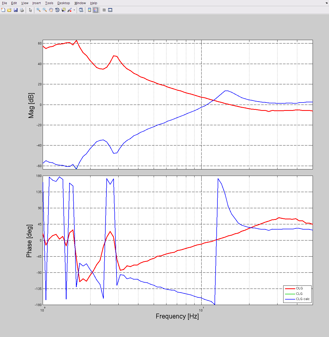
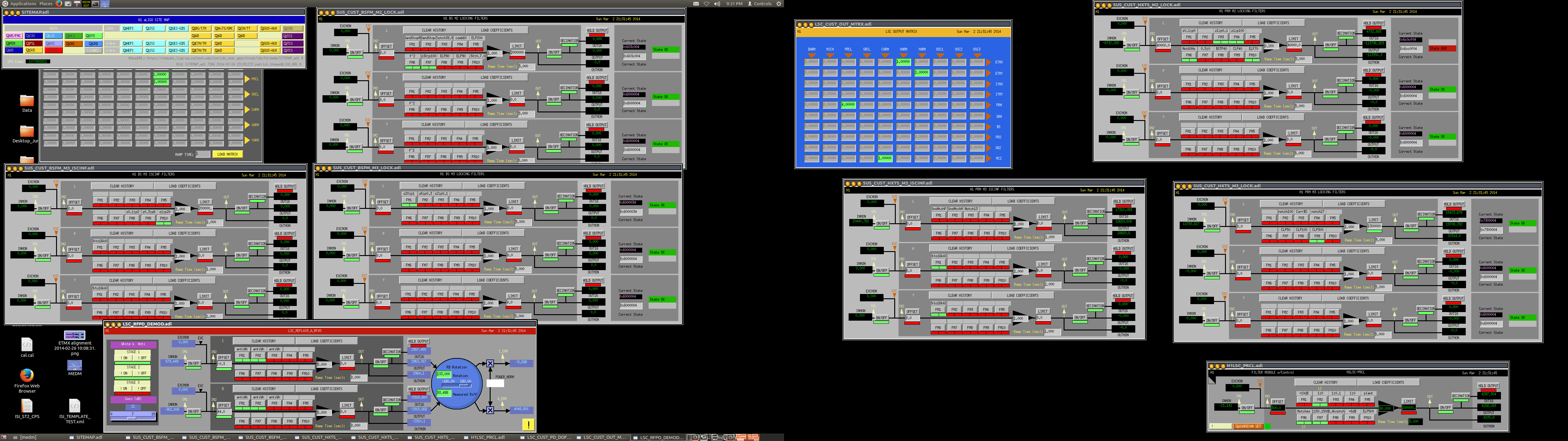
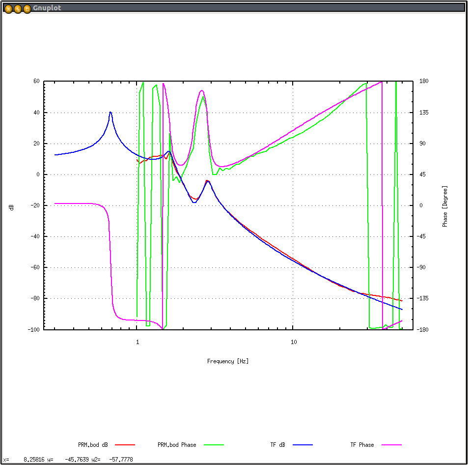
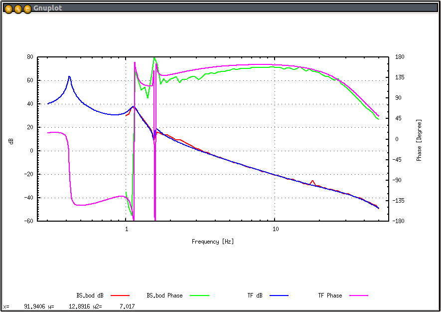
Kiwamu, Yuta, Stefan

Since all our OLG functions in PRMI never really made any sense, we locked PRY and carefully measured the actuation functions from BS to REFL_45_I and from PRM to REFL_45_I.

Plot 1 shows both BS and PRM transfer functions in ctsREFL45 / cts ISCinf drive (i.e. total actuation function). Both are closed loop corrected.
The BS makes sense: it is almost 1/f^2. I don't understand the PRM - need to sleep over it.

Plot 2 shows the OLG and the CLG.

Plot 3 is a snapshot of (almost) all relevant settings.

The data is in ~controls/sballmer/20140302:
BSdrive.xml
PRMdrive.xml
data/BS2REFL_mag_rad.txt
data/PRM2REFL_mag_rad.txt
data/plotIt.m

To do next:
-Understand PRM: for one we should check that the acquire mode TF of PRM M3 is as expected.
-Fit inverse actuation filters that make PRM and BS match
Stefan, Kiwamu
We then performed a fitting to get the zpk parameters out of the PRM actuator data. We used LISO. Here are the best parameters. We started from the HSTS suspension model, which was in the SUSsvn directory, as our initial guess. Since the data was not available at the low frequencies, we left the resonance at 68 mHz untouched.
=== fit parameters ===
zero 2.3327562304 7.4260090788 ### fitted (name = zero0)
zero 79.7052984298 ### fitted (name = zero1)
zero 7.1547795456 ### fitted (name = zero2)
zero 9.3953133943 ### fitted (name = zero3)
pole 2.8624375188 10.8992566943 ### fitted (name = pole0)
pole 1.6227455287 9.5958223237 ### fitted (name = pole1)
pole 6.839318e-01 2.754374e+01
factor 3.3153778483 ### fitted
We did the same fitting business on BS. We left the resonance at 42 mHz untouched.
=== fit parameters ===
zero 1.5468779344 47.4044594423 ### fitted (name = zero0)
pole 1.5752161758 20.5781923052  ### fitted (name = pole0)

	pole 1.1385114613 8.7983560598  ### fitted (name = pole1)


	# from BSFM model

	pole 4.201750e-01 3.057337e+01


	# from foton

	pole 37.5835 1.04298

	pole 104.999 0.95652

	pole 400

	pole 100


	zero 1.14018 0.814411

	zero 112.186 1e7

	zero 30


	factor 47.5420319676  ### fitted
Update on the PRM fitting:
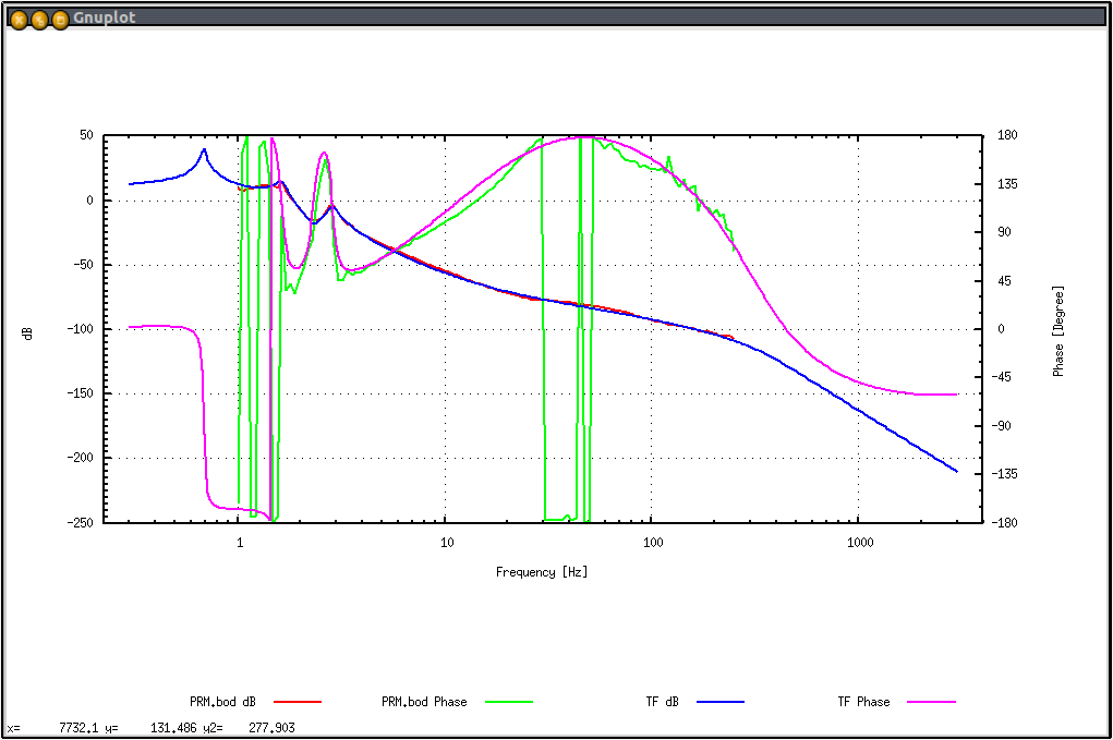
We took some more data points of PRM at higher frequencies to make the fitting more accurate at the high frequencies. We extended the swept sine to about 250 Hz.
Here are the new set of parameters:
=======================================
zero 2.3228474583 7.4113193282  ### fitted (name = zero0)

	zero 377.9190677283 41.5971099178m  ### fitted (name = zero1)

	zero 15.9199488645  ### fitted (name = zero2)

	zero 7.4012889472  ### fitted (name = zero3)


	pole 2.8669608985 10.2813809068  ### fitted (name = pole0)

	pole 1.6247562788 9.6336403562  ### fitted (name = pole1)

	pole 144.4376381898 487.5251791891m  ### fitted (name = pole2)

	pole 6.839318e-01 2.754374e+01


	# foton poles and zeros

	pole 314.966 0.95652


	factor 3.3634583469  ### fitted
I forgot to attach the plot.
We resolved the the non-sensical Q's below 0.5, removed a meaningless pole-zero pair and refitted. This tie we also added a small delay:

=======================================

zero 2.3543597867 8.0633003881  ### fitted (name = zero0)
zero 16.3221439613 855.9042353766m  ### fitted (name = zero1)
zero 3.5808330704  ### fitted (name = zero2)

pole 2.8457926226 10.9197851152  ### fitted (name = pole0)
pole 1.6165053404 8.7715269619  ### fitted (name = pole1)
pole 37.2960505517  ### fitted (name = pole2)
pole 6.839318e-01 2.754374e+01

# foton poles and zeros
pole 314.966 0.95652

delay 120u

factor 3.2012088652  ### fitted

=======================================

In foton:
zpk([0.139329+i*2.35023;0.139329-i*2.35023;9.53503+i*13.2475;9.53503-i*13.2475;3.58083],
   [0.130304+i*2.84281;0.130304-i*2.84281;0.092145+i*1.61388;0.092145-i*1.61388;
   0.0124154+i*0.683819;0.0124154-i*0.683819;37.2961],1,"n")

Its inverse (including a Q=1, f=1 pendulum):
=======================================
zpk([0.130304+i*2.84281;0.130304-i*2.84281;0.092145+i*1.61388;0.092145-i*1.61388;
    0.0124154+i*0.683819;0.0124154-i*0.683819;37.2961],
    [0.139329+i*2.35023;0.139329-i*2.35023;9.53503+i*13.2475;9.53503-i*13.2475;3.58083;
    0.5+i*0.866025;0.5-i*0.866025],1,"n")
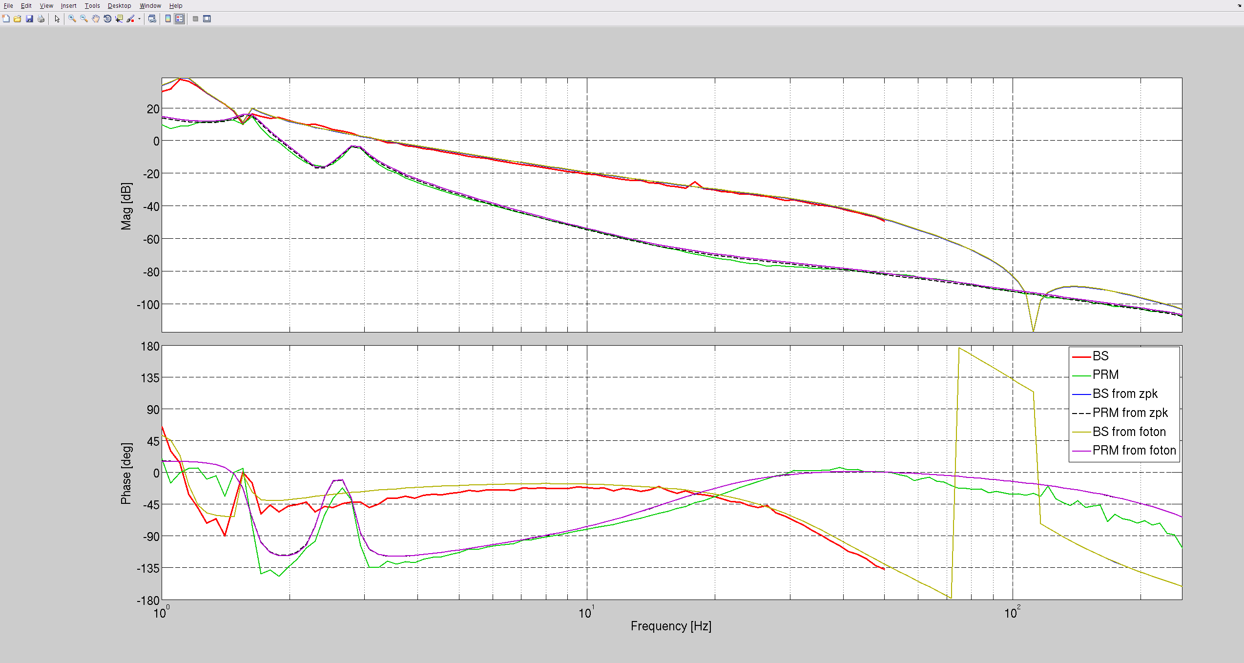
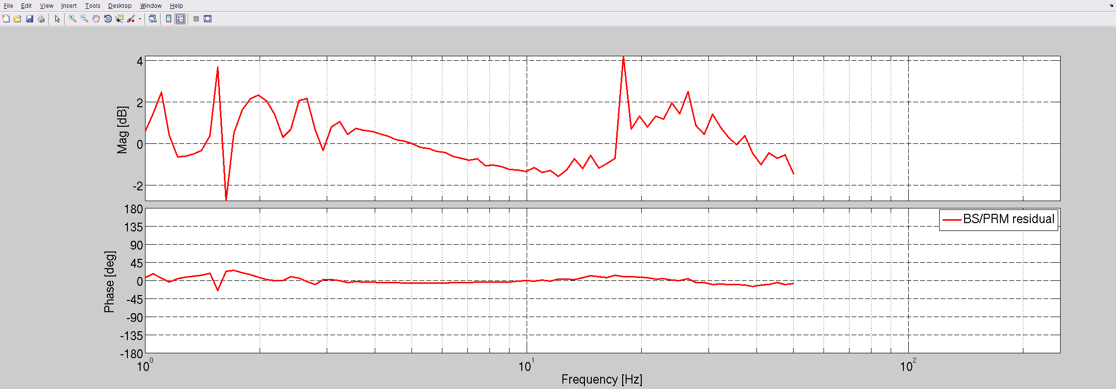
Attached is a plot of measured and fitted actuation functions for BS and PRM. Plot 2 shows the residual relative gain of BS/PRM - certainly a lot better than before...

Also, for completeness, here are the foton filters for the BS plant:

zpk([0.0163157+i*1.54679;0.0163157-i*1.54679],
    [0.0382738+i*1.57475;0.0382738-i*1.57475;0.0647002+i*1.13667;0.0647002-i*1.13667;
    0.00687158+i*0.420119;0.00687158-i*0.420119],1,"n")

as well as the inverse plant. Again, it includes a f=1Hz, Q=1 pendulum. Since the BS is 1/f^4, this also includes two 300Hz real poles as roll-off:

zpk([0.0382738+i*1.57475;0.0382738-i*1.57475;0.0647002+i*1.13667;0.0647002-i*1.13667;
    0.00687158+i*0.420119;0.00687158-i*0.420119],[0.0163157+i*1.54679;0.0163157-i*1.54679],1,"n")
zpk([],[0.5+i*0.866025;0.5-i*0.866025],1,"n")zpk([],[300;300],1,"n")