Inspired by Gabriele's fitting code for the nonstationary noise in DARM at L1 (for example, here), I tried performing a least-squares linear regression on the SPOP and SASY signals from Friday's long DRMI lock.  The motivation is to correlate the lower-frequency behavior of the DRMI to something that we can tune up in the ASC or SUS; this is distinct from Gabriele's code in that it doesn't consider the BLRMS in particular frequency bands (since I don't think we care too much about the noise in AS90 at 30Hz at the moment), and it looks over long timescales (which requires a lot of patience if you want to do it in DTT).

At the moment the code isn't as sophisticated as Gabriele's, for example it doesn't look at the square of the channels to find second-order couplings, and the channel ranking is sometimes a little suspicious.  But, it's in python.  :-)

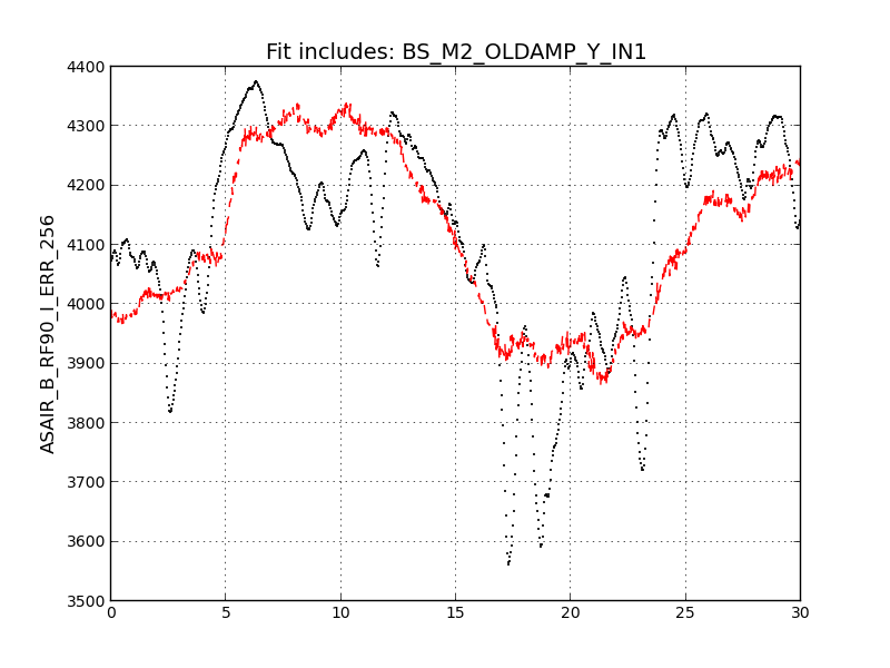
For Friday's lock, the channel that best explains the time-evolution of ASAIR_B_RF90 is the BS optical lever in yaw; this is demonstrated in the first plot with 30 seconds of data.  The fit in that plot only includes a first-order polynomial fit of BS_M2_OLDAMP_IN1 to the data, it's not perfect but it catches the low-frequency motion pretty well.  (This may already be academic, since the BS OL was tuned over the weekend.)

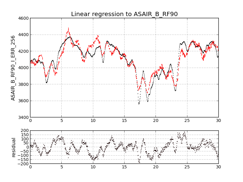
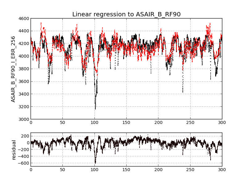
The second plot is a 30-second fit using 24 channels in the regression; things that were included are the LSC error signals, the ASC error signals (AS_A_RF36_I_PIT_OUT_DQ and so on), the BS, PR3, and SR3 optical levers (again, BS Yaw was the winner), and some ASC DC signals.  The fit isn't great but it kind of captures the excursions.  The third plot is 300 seconds of data.

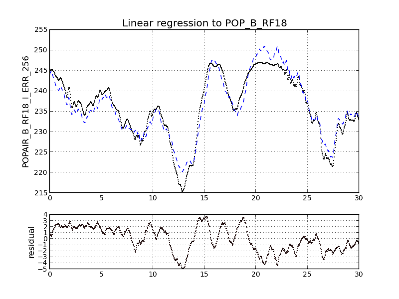
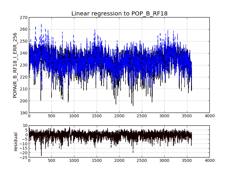
I also looked at POP18, this signal was correlated to the ASC-PRC1 error signal, REFL_A_RF9_I_{YAW,PIT}.  The fourth plot shows a fit to 30 seconds of data, the fifth plot is one hour of data.  Note that even though the fit coefficients are fixed values (not changing in time), the residuals are consistent over long timescales.

In all plots, the data we're fitting to is the black line, the fit result is the colored dashed line.  The x axis is in seconds.