Jim, Daniel

I calibrated the frequency of the CsIII Cesium Standard Atomic Clock in MSR by setting the Output Frequency on to 1 + (1010 * 10^-15). I did this at 12:26 PDT on July 2, 2015. I used the serial port on the back of the clock and the Monitor2 software installed on the IBM Thinkpad in MSR.

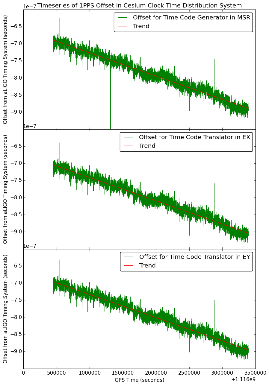
The previous setting was +1078 (parts per 10^15); I calculated the proper value to be 1010 (details below). I used the time difference between the atomic clock's 1PPS signals and our timing system's 1PPS signals. I took a linear regression to determine the rate of linear drift of the CsIII, since an improperly calibrated Cesium clock shows very little short-term jitter but does show long-term linear drift. Our timing system is long-term accurate since it's GPS backed.

I interpreted the meaning of the time difference according to an explanation from Daniel: a negative time difference means that the external (i.e. Cesium) 1PPS signal is ahead, while a positive time difference means it's behind. I calculated the drift rate to be approximately -6.8e-14 corresponding to -175 ns per 30-days.; the CsIII 1PPS is getting earlier and earlier relative to the timing system 1PPS, suggesting that the period is a bit short. I calculated the proper setting for the CsIII, as explained below, and talked to Microsemi's customer support to confirm that the CsIII's output frequency setting is what one would expect (the instructions were vague). He agreed with my interpretation but didn't have deep knowledge of the system. So we'll have to keep an eye out and check the drift rate in a few weeks to see if it is indeed close to zero (I expect it
will be fine).

The offset to be entered was calculated as follows. The current 1PPS period is given by tau_{measured} - 1 = m_{drift} where m_{drift} is the drift rate. If the clock's "natural" frequency is f_{natural}, then the current offset (Delta{f})_{measured} (which I found to be 1078 * 10^{-15} according to the Monitor2 interface) relates to the current measured period as (1 + (Delta{f})_{measured})f_{natural} = f_{measured} = frac{1}{tau_{measured}}. We want f_{calibrated} = 1, so we need to set (1 + (Delta{f})_{calibrated})f_{natural} = 1 = (1 + (Delta{f})_{measured})f_{natural}tau_{measured}, which simplifies to 1 + (Delta{f})_{calibrated} = (1 + (Delta{f})_{measured})tau_{measured}, giving (Delta{f})_{calibrated} = (1 + (Delta{f})_{measured})tau_{measured} - 1 = (tau_{measured} - 1) + (Delta{f})_{measured}tau_{measured}, or, in terms of the drift rate, (Delta{f})_{calibrated} = m_{drift} + (Delta{f})_{measured}(1 + m_{drift}), which we then divide by 10^{-15} in order to get the value to be entered into the Monitor2 software. See the attached code (written in Julia) for the precise method used. The output (besides the graphs, also attached) includes the above calculations:

Drift rate in Time Code Generator in MSR: -6.786047272268983e-14
Drift rate in Time Code Translator in EX: -6.788794482601771e-14
Drift rate in Time Code Translator in EY: -6.780539996010063e-14
mean_drift_rate = mean($(Expr(:comprehension, :(channel.drift_rate), :(channel = channels)))) => -6.785127250293606e-14
delta_f_measured = 1.078e-12 => 1.078e-12
delta_f_calibrated = mean_drift_rate + delta_f_measured * (1 + mean_drift_rate) => 1.0101487274969909e-12
what_to_enter_into_monitor2 = delta_f_calibrated / 1.0e-15 => 1010.1487274969908

Note that the drift rates calculated for each channel are in very close agreement. I used this to pick the new setting of 1010 for the Cesium clock. The channels I looked at were:

H1:SYS-TIMING_C_MA_A_PORT_2_SLAVE_CFC_TIMEDIFF_1 (Time Code Generator in MSR)
H1:SYS-TIMING_X_FO_A_PORT_9_SLAVE_CFC_TIMEDIFF_1 (Time Code Translator in EX)
H1:SYS-TIMING_Y_FO_A_PORT_9_SLAVE_CFC_TIMEDIFF_1 (Time Code Translator in EY)

The timeseries (with linear regressions) and histograms are included. The period analyzed is from the beginning of ER7 until last week. I had to remove a chunk of spurious data from the EY channel since Dave and I were using the BNC cable for a different test and polluted the EY channel during that time.

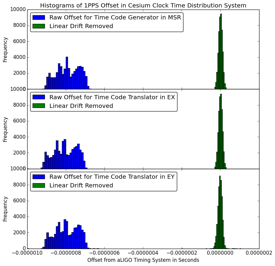
The linear regression shows a very clear and steady trend, as expected. Standard deviation of the atomic clock offset is reduced by a factor of five once linear drift is accounted for, and the histogram more closely follows a Gaussian distribution:

std(z) => 1.1845358220722136e-8    # Jitter about linear trend
std(y) => 5.853090568967089e-8      # Absolute time difference