kiwamu.izumi@LIGO.ORG - posted 22:06, Friday 07 August 2015 - last comment - 09:25, Tuesday 11 August 2015(20334)
Pcal now uses sus dynamical models
The Pcal RX and TX photodetectors now have filters which simulate the suspension dynamical response in order to convert the signals into displacements. The filters are installed and enabled.
Since each signal chain is whitened, one needs to apply two poles at 1 Hz with a gain of 1 when using these signals.
[Background]
Traditionally Pcal uses a free-mass approximation for the suspension responses which is a simple 1/f^2. This can introduce undesired inaccuracy at low frequencies. Even though we know the accuracy is not too terrible at around 30 Hz, where the lowest frequency Pcal lines are, we decided to replace the old 1/f^2 approximation with the dynamical suspension model.
[Tagging suspension models]
Prior to the update of the filters, we take this opportunity to tag our suspension models. As usual, I used Jeff's code to create tags. The scripts is in:
/ligo/svncommon/SusSVN/sus/trunk/Common/MatlabTools/tagsusdynamicalmodel.m @rv7754
Also, I updated h1etmx.m which is a parameter file dedicated for creating the h1etmx suspension model. I only updated the fundamental violin mode. I confirmed that the mass was correct since this is critical for Pcal. As for h1etmy.m, it was already good from the beginning. The mass is correct and the violin modes are specified up to 8th harmonics. So I did not update it.
The tagged models are now in SVN:
- quadmodelproduction-rev7652_ssmake4pv2eMB5f_fiber-rev3601_h1etmx-rev7641_released-2015-08-07.mat
- quadmodelproduction-rev7652_ssmake4pv2eMB5f_fiber-rev3601_h1etmy-rev7640_released-2015-08-07.mat
[Script does all at once]
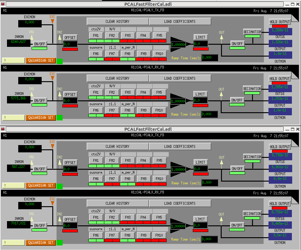
I wrote a matlab script which picks up the tagged suspension models and subsequently quack them into the Pcal TX and RX PD filters. For convenience, the suspension responses are divided into three pieces -- normalized suspension response, zpk([], [1,1], 1, "n") and DC gain in [m/N]. Combining all three makes the complete suspension response. The normalized suspension response has a gain of 1 at DC (technically speaking at 10 mHz) and all the zeros and poles except for two poles at 1 Hz. The two-pole filters are intentionally turned off in order to whiten the whole signal chain. Therefore one has to apply the two poles when calibrating the signals. The attached is a screen shot of how they look in the medm screens.
The script can be found at
/ligo/svncommon/CalSVN/aligocalibration/trunk/Runs/PreER8/H1/Scripts/Pcal/quad_response.m
/ligo/svncommon/CalSVN/aligocalibration/trunk/Runs/PreER8/H1/Scripts/PcThe Pcal RX and TX photodetectors now have filters which simulates the suspension dynamical response in order to convert the signals into displacements. The filters are installed and enabled.
Since each signal chain is whitened, one needs to apply two poles at 1 Hz with a gain of 1 when using these signals.
[Backgrounds]
Traditionally Pcal uses a free-mass approximation for the suspension responses which is a simple 1/f^2. This can introduce undesired inaccuracy at low frequencies. Even though we know the accuracy is not too terrible at around 30 Hz, where the lowest frequency Pcal lines are, we decided to replace the old 1/f^2 approximation with the dynamical suspension model.
[Tagging suspension models]
Prior to the update of the filters, we take this oportunity to tag our suspension models. As usual, I used Jeff's code to create tags. The scripts is in:
/ligo/svncommon/SusSVN/sus/trunk/Common/MatlabTools/tagsusdynamicalmodel.m @rv7754
Also, I updated h1etmx.m which is a paramter file dedicated for creating the h1etmx suspension model. I only updated the fundamental violin mode. I confirmed that the mass was correct since this is critical for Pcal. As for h1etmy.m, it was already good from the beginning. The mass is correct and the violine modes are specificed up to 8th harmonics. So I did not update it.
The tagged models are now in SVN:
quadmodelproduction-rev7652_ssmake4pv2eMB5f_fiber-rev3601_h1etmx-rev7641_released-2015-08-07.mat
quadmodelproduction-rev7652_ssmake4pv2eMB5f_fiber-rev3601_h1etmy-rev7640_released-2015-08-07.mat
[Script does all at once]
I wrote a matlab script which picks up the tagged suspension models and subsequently quack them into the Pcal TX and RX PD filters. For convenience, the suspension responses are divided into three pieces -- normalized suspension response, zpk([], [1,1], 1, "n") and DC gain in [m/N]. Combining all three makes the complete suspension response. The normalized suspension response has a gain of 1 at DC (technically speaking at 10 mHz) and all the zeros and poles except for two poles at 1 Hz. The two-pole filters are intentionally turned off in order to whiten the whole signal chain. Therefore one has to apply the two poles when calibrating the signals. The attached is a screen shot of how they look in the medm screens.
The can be found at
/ligo/svncommon/CalSVN/aligocalibration/trunk/Runs/PreER8/H1/Scripts/Pc
Images attached to this report
Comments related to this report
Prior to this change, photodiodes (TX and Rx PD) calibartion coeffcient were reported in metres/Volt *(1/f^2). Now with the suspension model in place, we have calibrated the photodiodes in terms of Force Coefficient (N/V). The filter banks, as shown in the attachement above, now reflect these new N/V calibration factors. Appropriate changes have been made to the DCC document (T1500252) as well.
This is an additional note about the quack function -- when I was using quack, I had a difficulty in quacking an state-space suspension model into a foton filter. See the detail below.
In matlab, I had been using something like:
quad.d = minreal( zpk( c2d(quad.ss, smaplingTime, 'tustin' ), tolerance )
where
quad.ss is a state-space representation of the quad suspension response, and samplingTime in this case is 1/16384 sec. The reason why I used the minreal function is that otherwise it would come with too many number of poles and zeros which exceeded the number of poles and zeros that foton can handle. I tried adjusting the tolerance of minreal in order to reduce the number of poles and zeros, but it was extremely difficult because it ended up with either too many poles/zeros or too few poles and zeros.
Instead, I tried the following command which at the end worked fine:
quad.d = c2d( minreal( zpk(plant.ss), tolerance ), samplingTime, 'tustin');
The combination of the functions are exactly the same, but the ordering is different. It does
minreal before c2d. This allowed me for having a reasonable number of poles and zeros.