CAL CS suspension filters are ready to go

As Jeff reported yesterday (alog 21280), we have completed the assessment of the suspension scaling factors. In order to finish up the suspension side of the calibration, all we needed to do is to update the CAL CS filters that should accurately simulate the latest suspension transfer functions. So I implemented and tested the new filters today. It seems good so far -- no strange specral shape or drastic change in the DARM strain curve were seen as expected. The filters are ready to go.

The screen shot attached below is a quick comparison of the calibration -- the blue curve is with the old ER7 suspension filters engaged and the red curve with the new ER8 suspension filters engaged. As shown in the plot, there is no big difference as expected. Unfortunately since the low frequency components below several 10 Hz seemed to be sufficiently non-stationary that it does not allow us to make accurate comprasion between the old and new filters in this way.

 

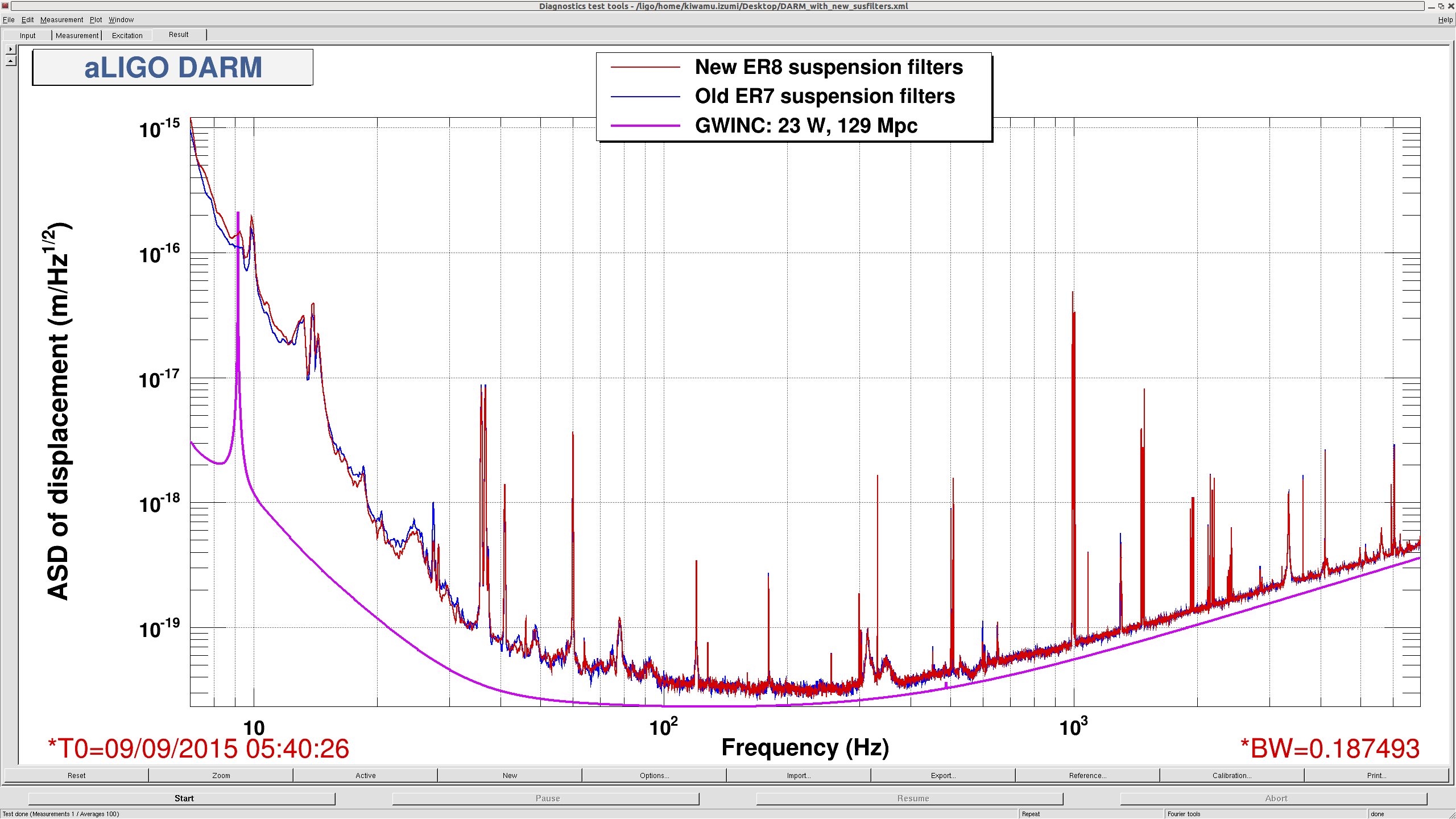
CAUTION: The new suspension filters will not be enabled until the calibration filters on the sensing side are installed; CAL CS will keep using the old ER7 suspension filters for now.

 

---

(Overview and implementation process)

The implementation of the suspension filters has been done in the order of

1. Obtain the latest suspension model.
2. Convert the suspension responses into discretized model such that the CAL CS can handle
3. Run autoquack to implement the discretized models into CAL CS.
4. Copy  the digital control filters, such as ETMY_L3_LOCK_L and so forth, to CAL CS

Step 1, 2 and 3 are done by a single matlab script which can be found at:

aligocalibration/trunk/Runs/ER8/H1/Scripts/CALCS/quack_eyresponse_into_calcs.m

The script calles H1DARMOLGTFmodel_ER8.m at first in order to collectively obtain all the up-to-date parameters. Subsequently it extracts the necessary suspension responses and convert them into discretized filters. The way we handle the suspension filters are described in the next section. Once the filters are in the discrete format, then the script runs autoquack to directly edit the foton file of CAL CS.

Step 4 is done by a different script;

aligocalibration/trunk/Runs/ER8/H1/Scripts/CALCS/copySus2Cal.py

It  simply copies the relevant parts of H1SUSETMY.txt to H1CALCS.txt. There is one exception that is FM1 of ETMY_L1_LOCK_L which caused a trouble before (alog 20700 and alog 20725). The script is now coded such that it modifies this particular filter and gets rid of the integrator. I followed our latest approach that is to replace the filter module with zpk([0.3], [0.01], 30, "n") as described in alog 20725. Optionally, one can run a python script which turns on the necessary switches and filters in CAL CS. The script can be found at

aligocalibration/trunk/Runs/ER8/H1/Scripts/CALCS/setCalcsEtmy.py

Right now, both python scripts edit the ITMY part of CAL CS instead of the ETMY part so that we can make a comparison between them -- the ITMY signal paths represent the new suspension filters while the ETMY paths still uses the old ER7 filters.

 

(Accuracy of the suspension responses)

One of the tricky parts in implementing the suspension filters into a front end model is that we have to pay attention to how accurately the front end can mimic the suspension responses. There are practical limitations associated with this issue. For example, a single filter module can not handle more than 10 SOS segments. Also, the distortion of the filter is inevitable (see for example G1501013 ) because of the finite sampling rate. So it is extremely important to check if the installed filters are accurate.

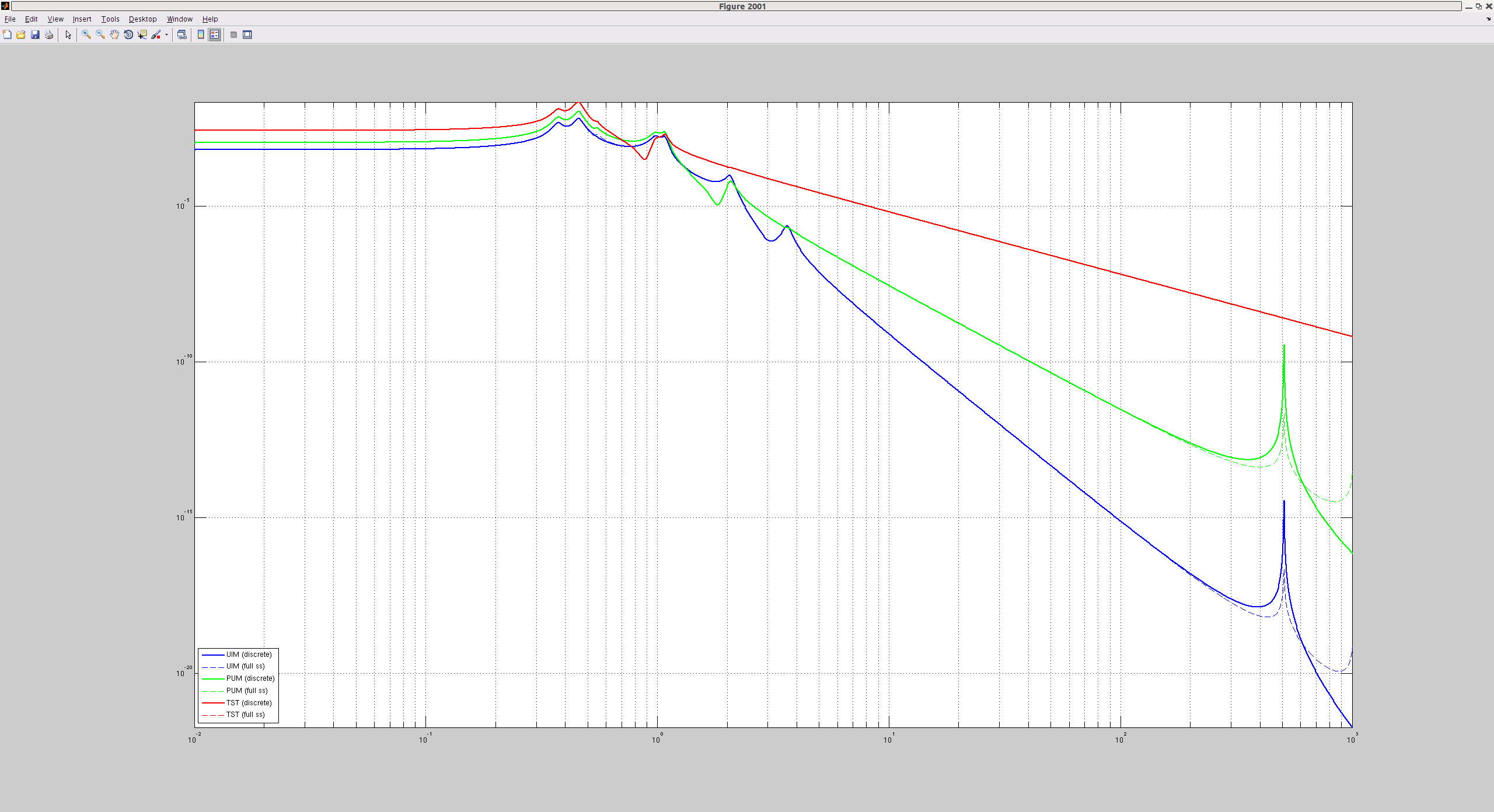
In order to asses the accuracy, I made a comparison between the discrete suspension responses and the state-space full suspension model. The plot shown right below is a plot of the transfer functions only in magnitude. The dashed lines are the full state space models that we are trying to mimic and the solid lines are the resultant direcrete models. As one can see, the TST stage looks accurate as the dashed and solid curves are almost completely on top of each other. On the other hand the PUM and UIM stages have a big difference as they go to high frequencies. This is due to compromize for the extremely high-q violin modes and I will explain this in the next section. Apart from the violin modes, UIM had the largest decrepancy at around the mechanical resonances, in 0.3 - 1 Hz. By the way the y-axis is meant to be m/N.

If we take ratio of (discrete transfer function) / (full state space model), it is going to look like this:

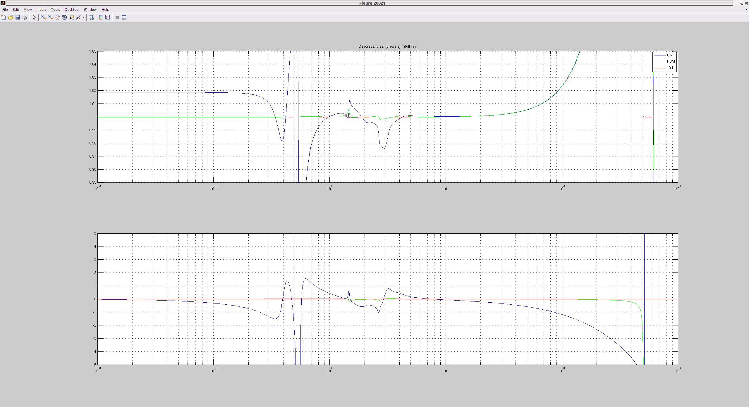
As mentioned earlier, the TST stage is very accurate across the entire frequency band. On the other hand, the PUM and UIM deviate from the full state space models as they go to high frequencies. Even though they both deviate from the full ss models by 2.4 % at 100 Hz and 0.2 % at 30 Hz in magnitude, this is already good enough. PUM is the leading-actuator in a band of 1-30 Hz and that is the band where the PUM is accurate at a sub-pecent level. UIM takes care frequencies below 1 Hz and does not really matter above 1 Hz, although I made a slight hand tweak as described in a subesequency section in this alog. Overall, this result is satisfying.

 

(Violine modes' Q are intentionally lowered)

The current full ss suspension model assumes Q of the violine modes to be on the order of 1e9. Regardless of whether it is accurate or not, it is not a good idea to directly implement such filters in a front end. If they were implemeted with such a high Q, their impulse respones would last forever. Also, the resonance is so tall that any kind of numerical precision error would ring it up. Anyway, I did not like the high-Q filters and therfore artificially lowered their Q's to 1e3 such that they damp on a time scale of a few seconds. At the beggining, I tried completely getting rid of the violin modes, but this turned to be a bad idea because they produced a large descrepancy in PUM by 1 or 2 % at 30 Hz where the accuracy matters. So instead, I decided to keep the vilone modes but with a much lower Qs.

I edited quack_eyresponse_into_calcs.m such that it automatically detects high-Q components and lowers the Q to a user-specified value. Also, the code still internally keeps the high-Q version of the filters and therefore switching back to high-Q is trivial (if necessary in future). This lower-Q modification is applied in PUM and UIM.

 

(A compromise factor in UIM)

There was another trick. Since UIM needed more poles and zeros than TST and PUM do, it was difficult to simulate the UIM mechanical response in a single filter module. I could have split it into multiple filter banks, but as UIM does not really impact on the calibration, I decided to go with a single filter module. I decreased the number of zeros and poles by running matlab's minreal with a high tolerance and it resulted in frequency-dependent inaccuracy as shown in the above plots. In addition to the frequency dependent components, the response in a band of 1-30 Hz became lower than that of the full ss by roughly 2%. Even though this does not matter, I decided to raise the discrete response by multiplying an extra scale factor such that the UIM is accurate in 1-30 Hz band for completeness.

(A coarse comparison between ER7 and ER8 suspension filters)

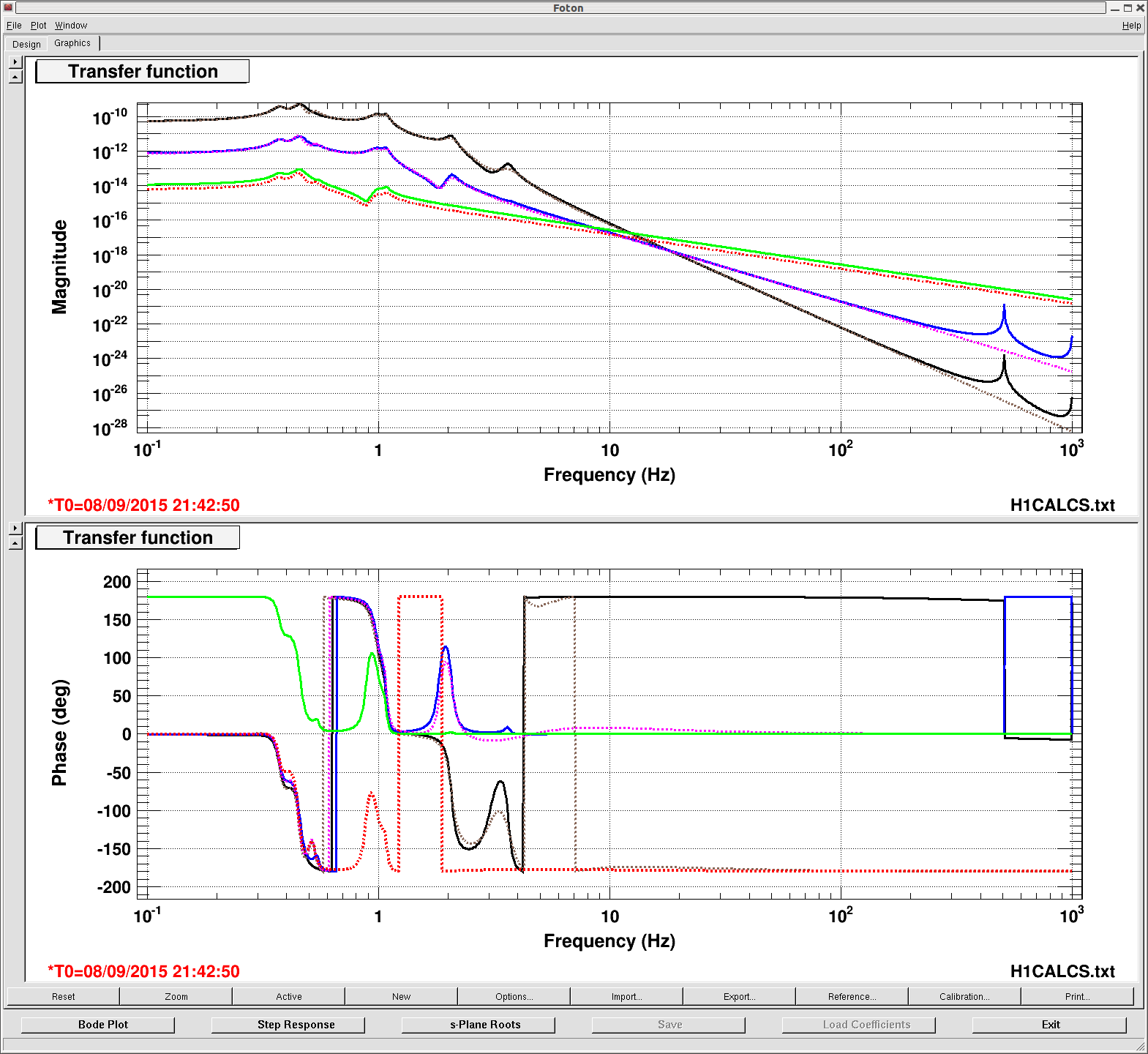
This is a screenshot of foton comparing the suspension filters from ER7 and the ones for ER8.  The black solid, blue solid and green solid lines are the new UIM, PUM and TST filters in meters/counts respectively. The dashed lines are the old ER7 suspension filters. There are some remarks:

• TST now contains the negative sign within the filter module, which made a 180 deg phase shift. So we can now get rid of the negative gain from CAL-CS_DARM_ANALOG_ETMY_L3_GAIN
• TST is higher than it used be by 45 % as described in Jeff's alog 21280.
• PUM and UIM are slight increased as described in alog 21280.
• PUM and UIM now contain violin modes (actually the screenshot was taken before I lowered the violin Qs and therefore they are as high 1e9 in the screen shot.)
• The mechanical resonances at around 1 Hz are now more up-to-date and should be more accurate.

 

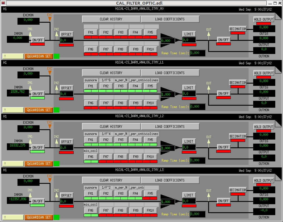
(Implemented filters)

Here is a screen shot of the filter modules for the new suspension responses in CAL CS. Currently they are installed in the ITMY filter modules for convenience. The suspension filters are split into multiple modules as described in the followings.

• FM1 = normalized suspension with the DC gain normalized to 1. This is the same idea as Pcal calibration filters (alog 20334).
• FM2 = de-whitening filters. Together with FM1, they will make a frequency dependent part of the suspension responses with the DC gain normalized. Note that they don't have vilolin modes which will be added at FM5
• FM3 = scaling factor which converts signals from Newton to meter. This is common to Pcal.
• FM4 = another scaling factor which converts signals from counts to Newton.
• FM5 = violin modes, applicable only in L1 and L2 stages.
• FM6 = coil mismatch as described in alog 21275