GregM, RickS, DarkhanT, JeffK, SudarshanS
This was an attempt to study what the GDS output will look like with kappa factors applied. GregM volunteered to create test data with kappa applied, kappa_C and kappa_tst, on 'C01' data for the days between October 1 through 8. The kappa corrected data is referred as 'X00'. The correction factors are applied by averaging the kappa's at 128s. This was loosely determined from the study done last week (alog 22753) on what the kappa's look like with different time-averaging duration.
Here, comparisons are made between 'C01' as 'X00'. The first plot contains the kappa factors that are relevant to us. kappa_tst and kappa_C are applied and are thus relevant, whereas cavity pole (f_c) varies quite a bit at the beginning of each lock-stretch and is thus significant but we don't have an infrastructure to correct it. The first page contains kappa's calculated at a 10s FFT and is plotted on red and a 120s averaged kappa's plotted in blue. Page 2 has similar plot but has kappa plotted at 20 minutes averaging (it helps to see the trend more clearly).
Page 3 and onwards has plots of GDS/PCal at pcal calibration line frequencies for both magnitude and phase plotted for C01 and X00 data. The most interesting plots are the magnitude plots because applying real part of kappa_tst and kappa_c does not have a significant impact on phase. The most interesting thing is that applying kappa's flattens out the long-term trends in GDS/Pcal in all four frequencies. However, at 36 Hz, it flattens out the initial transient as well but introduces some noise into the data. At 332 Hz and 1 Khz it introduces the transient at the beginning of the lock stretch and it does not seem to have much effect at 3 KHz line. We think that this transient should be flattened out as well with the application of kappa's. The caveat is we don't apply cavity pole correction and we know that the cavity pole has a significant effect in the frequency region above the cavity pole.

DarkhanT, RickS, SudarshaK
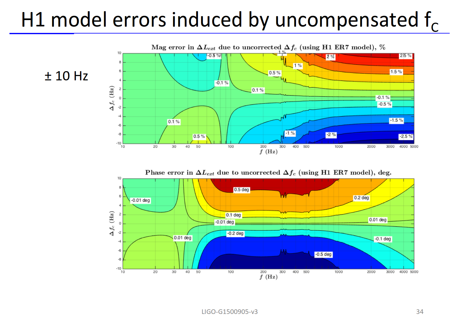
After seeing the ~2 % transient at the beginning of almost each lock stretch in GDS [h(t)] trend at around 332 Hz, we had a hunch that this could be a result of not correcting for cavity pole frequency fluctuation. Today, Drarkhan, Rick and I looked at old carpet plots to see if we expect variation similar to what we are seeing and indeed the carpets plot predicted few percent error in h(t) when cavity pole is varying by 10 Hz.
So we decided to correct for the cavity pole fluctuation to h(t) at calibartion line frequency. We basically assumed that h(t) is sensing dominated at 332 Hz and used absolute value of the correction factor that change in cavity pole would incur [C/C' = (1+ i* f /f_c)/(1+ i* f /f_c')] and appropriately multiplied it to the GDS output.
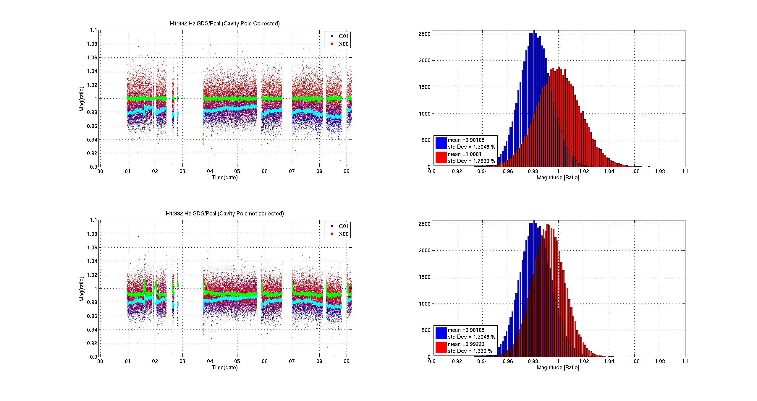
The result is attached below. Applying cavity pole fluctuation gets rid of the transient seen at the beginning of each lock stretch as well as 1 % overall systematic we saw on the whole trend. We used cavity pole as 341 Hz for nominal value which is calculated from the model at the time of calibration. In the plot below, the cyan in both bottom and top left are the output of GDS CALIB_STRAIN/ PCAL uncorrected for Kappas, the green on the top left is corrected for kappa_tst, kappa_C and cavity pole whereas the green on the bottom left is corrected for kappa_C and kappa_tst only ( we only know how to correct these in time domain).