Evan G., Jeff K.
Revisiting measurements Jeff made in the field [1],[2],[3] and new measurements with those I took in the EE lab, we compared with the UIM residuals measurements obtained using the Pcal and ALS DIFF measurements. Attached is a figure showing the electronics chain and comparing with the residuals obain. We find that the BOSEM electronics account for some of the residuals found in the UIM measurements, but not all. At this point, we have only clues, but no solid evidence for what remains of the residuals. We have three theories:
- UIM to TST mechanical dynamics are not modeled correctly. Violin mode frequencies are PUM --> TST frequencies [~505, 1k, 1.5k, etc.] from G1501372, page 5, but shouldn't they be UIM to PUM mode frequencies [~420, 800, 1.6k, etc.]?
- We are missing some frequency response in the actuator. We had been claiming it is the inductance but the attached plot shows that it is not enough. Is there some frequency dependence in the actuation from the BOSEM? Maybe the old "cross-coupling" effect of the BOSEM from the TOP-2-TOP mass transfer functions?
- Is there a flaw in the (PCAL/DARM) x (DARM/UIM) / Model measurement?
I set up in the EE shop a UIM driver, satellite box, and BOSEM to repeat Jeff's measurements and verify we observe the same effects. Indeed, I observed similar issues that Jeff had observed in his measurements from the floor. We put these measurements on top of the UIM actuation residuals measurement/model but, unfortunately, find that they are not completely accounted for by the electronics chain.
We started to think about what else could be going wrong with the residuals, but so far have come up with the only three theories above. To undertand this effect in more detail, Jeff is currently undertaking exploratory measurements of the UIM-->DARM and Pcal-->DARM to frequencies higher than 100 Hz. Hopefully these measurements will shine some light on this effect.

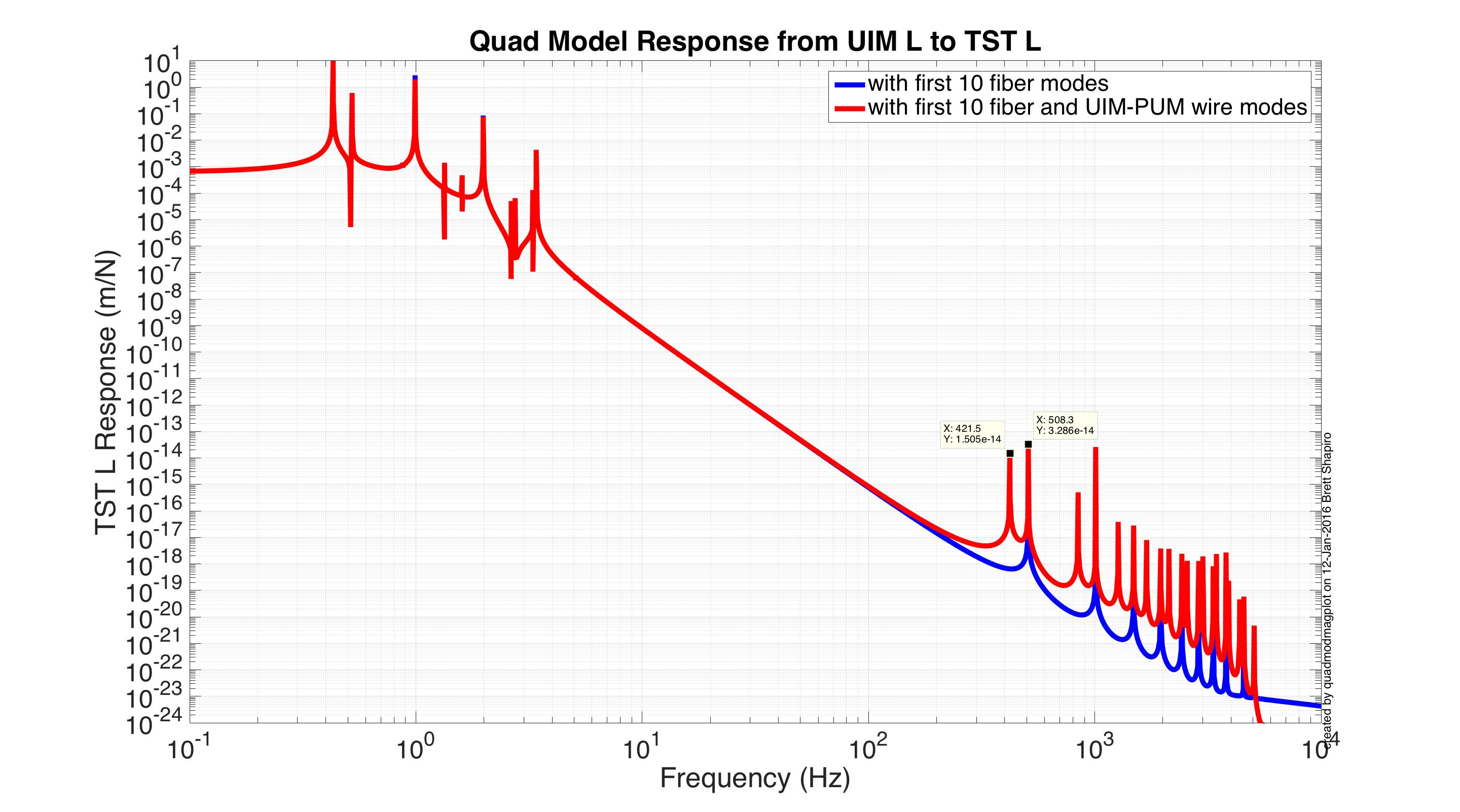
The quad model on the svn does not have UIM-PUM wire violin modes. I just drafted an update that does include these, which I used to generate the attached figures. I'll commit this update if it appears consistent with measurements.
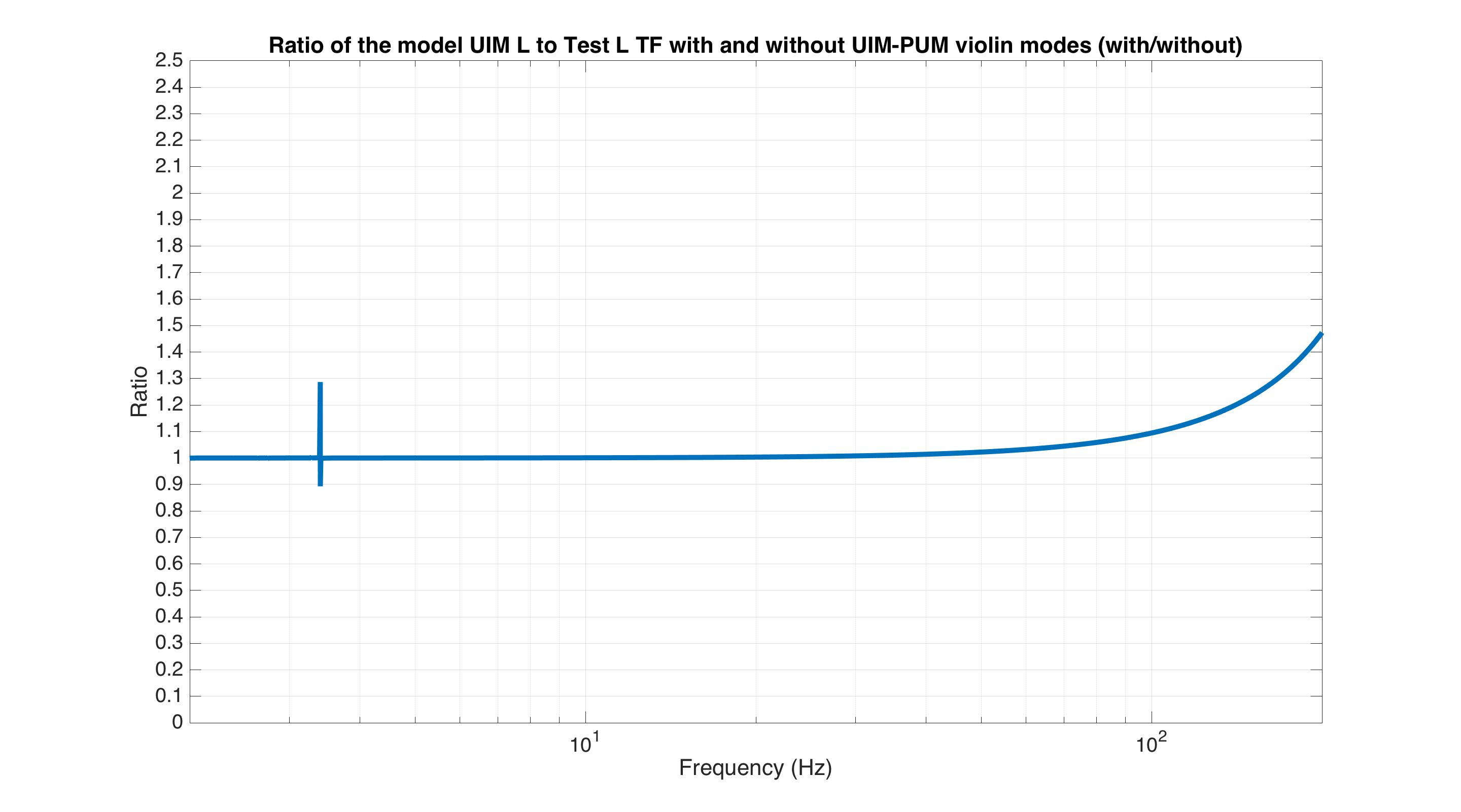
The plot ViolinModes_12Jan2016.jpg compares the model UIM L to Test L transfer function with and without the UIM-PUM modes, but with the fiber modes in both cases. I guessed the UIM-PUM violin modes to be a Q of 100,000, but that could be off an oder of magnitude or two. The second figure plots the ratio of these 2 transfer functions.
According to this second figure, the UIM-PUM violin modes explain some, but not all of the discrepancy seen between the measurements and the model in the log above. So either the model is not correct, or there is still something in the feedback loops we are missing.
For the Bench measurements, the data is stored at:
/ligo/svncommon/CalSVN/aligocalibration/trunk/Runs/PostO1/H1/Measurements/Electronics/BenchUIMDriver/2016-01-12
Attached are plots showing the individual components of the coil driver electronics fitted with the vectfit program in Matlab and using LISO. I report the fitted LISO values below with respective uncertainties.
Dummy BOSEM connected, with output impedance network (see figure UIM_out_impedance.pdf):
Best parameter estimates:
zero0:f =  84.1507169277 +- 1.627 (1.93%)
pole0:f =  303.5726548020 +- 5.431 (1.79%)
pole1:f =  127.6915337428k +- 3.535k (2.77%)
factor =  2.2065872530m +- 17.45u (0.791%)
This fit shows the calibration of 2.2 mA/V, one zero at 84.15 Hz, and two poles at 303.57 Hz and 127.7 kHz.
BOSEM only (output impedance network divided out so only BOSEM transfer function remains, see figure UIM_bosem.pdf):
Best parameter estimates:
zero0:f =  334.8526120460 +- 3.892 (1.16%)
zero1:f =  1.2383234778k +- 43.39 (3.5%)
zero2:f =  8.2602408615k +- 320.8 (3.88%)
pole0:f =  747.0160319882 +- 27.6 (3.69%)
pole1:f =  5.3613221192k +- 210.2 (3.92%)
pole2:f =  25.8483289876k +- 310.1 (1.2%)
pole3:f =  232.8627791989k +- 3.041k (1.31%)
factor =  11.6075630096m +- 14.92u (0.129%)
For some reason, this transfer function is tricky to fit. These are the fewest number of zeros and poles I could put in LISO and still provide a good fit to the data. LISO does complain that strong correlation exists between pole1<-->zero2 and pole0<-->zero1. When I removed these pairs, the fit became much worse, so I left them in.
As a comparison with the full chain: digital AntiAcq x analog Acq (output impedance network) x BOSEM (see figure UIM_full.pdf). The model fits the measurement with 2% up in magnitude to 40 kHz, and within 1 degree in phase up to 50 kHz.
Finally, the previously shown plot in the original post divides out the full BOSEM measurement in the field ('field BOSEM'), but the model already takes care of the analog output impedance network, so this original plot was double-counting. I attach here a corrected version of the plot (see UIM_res_with_elec.pdf). This shows that the BOSEM does indeed correct for some of the excess residual, it is not the dominant contributor to the behaviour above ~60 Hz.