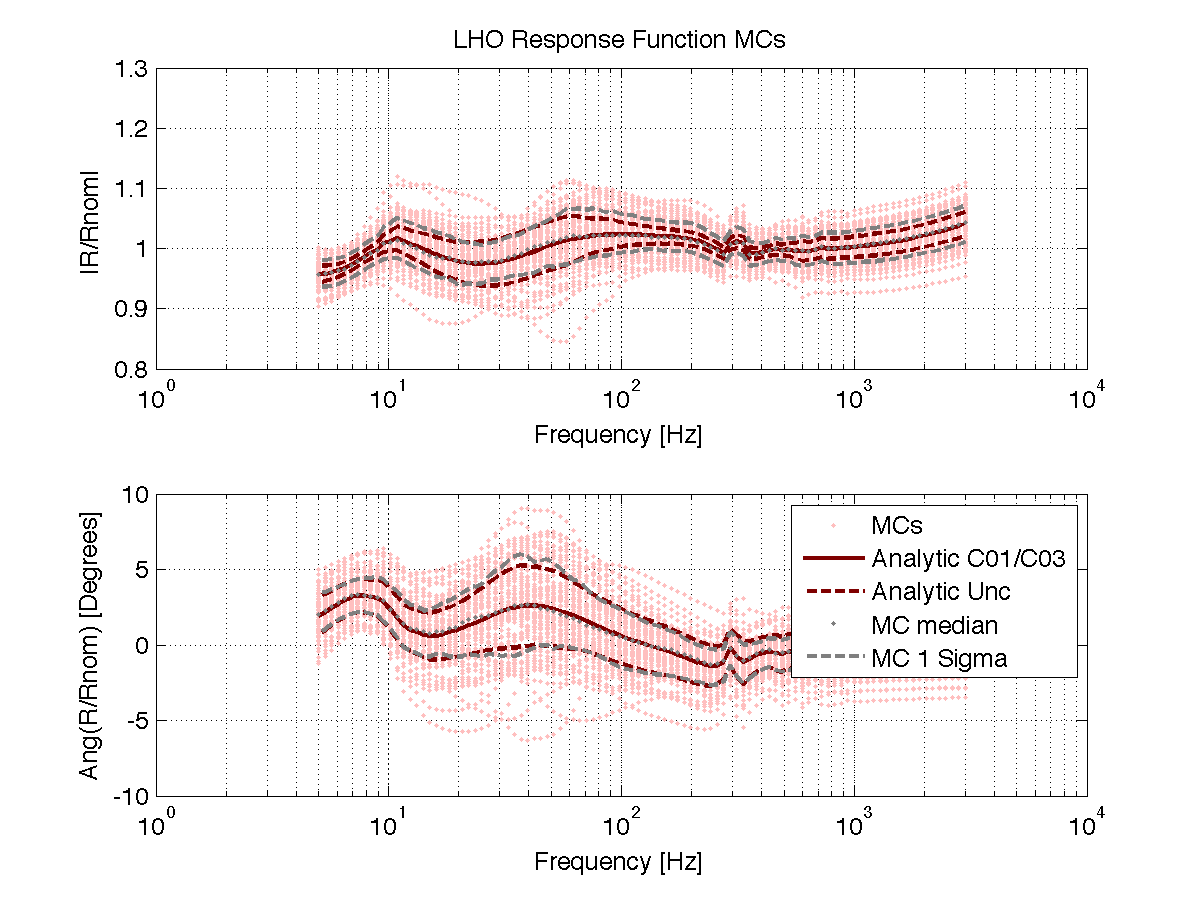
C. Cahillane

I have been working on a preliminary calibration uncertainty budget for the parameter estimation group to come up with something more sophisticated than "10% and 10 degrees" spline fitting that is currently done.

The plot below shows my attempt at a numerical budget.  I have imported my analytical budget for simplicity of comparison.  They are the dark red lines.  Dashed lines represent the uncertainty envelope.  
What is plotted is the C01/C03 response function.  The deviations from 1 (mag) or 0 (phase) represent the systematic differences between our model and our measurements between our C01 (uncorrected) and C03 (perfect) calibration versions.
The light red dots illustrate the 100-iteration MC performed.  
These MCs were performed in the following way: The response function is a function of 14 parameters [R(f) = R(f|a1,a2,a3,...,a14)].  Each of these a_i have an associated uncertainty sigma_a_i.  
The person running the MC supplies 14 random samples from a 0-mean 1-std Gaussian distribution.  I take these random samples, multiply it by sigma_a_i, then alter a_i by the result [a_i_new = a_i + rand * sigma_a_i].  Then I recalculate the response function using a_i_new.  That gives me a single light red line.

The dark grey lines are the median (dots) and 1 sigma deviations from the median.  The deviations are found by looking for the 68% confidence interval.  For example, in this 100 iteration example, I look for the innermost 68 points and plot the limits on this as my "numerical envelope".  This envelope agrees fairly well with my analytical envelope.  If I increase the number of iterations the envelope should collapse to my analytical uncertainty envelope.

See the LLO Numerical Uncertainty Budget (LLO aLOG 25104)