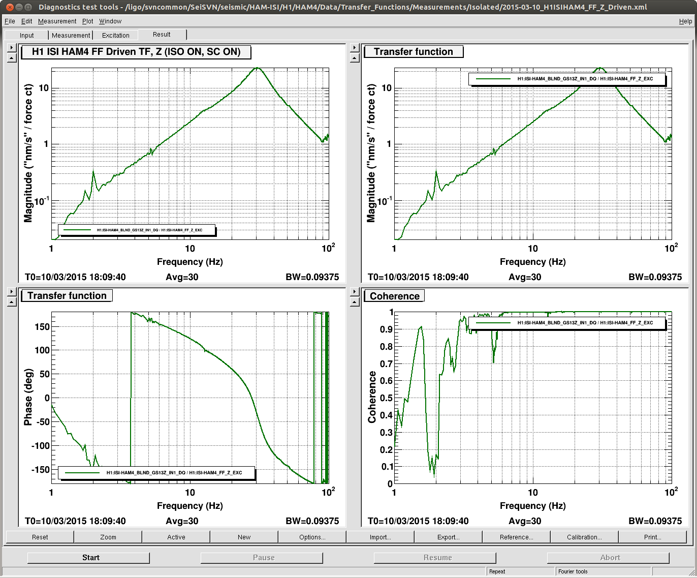
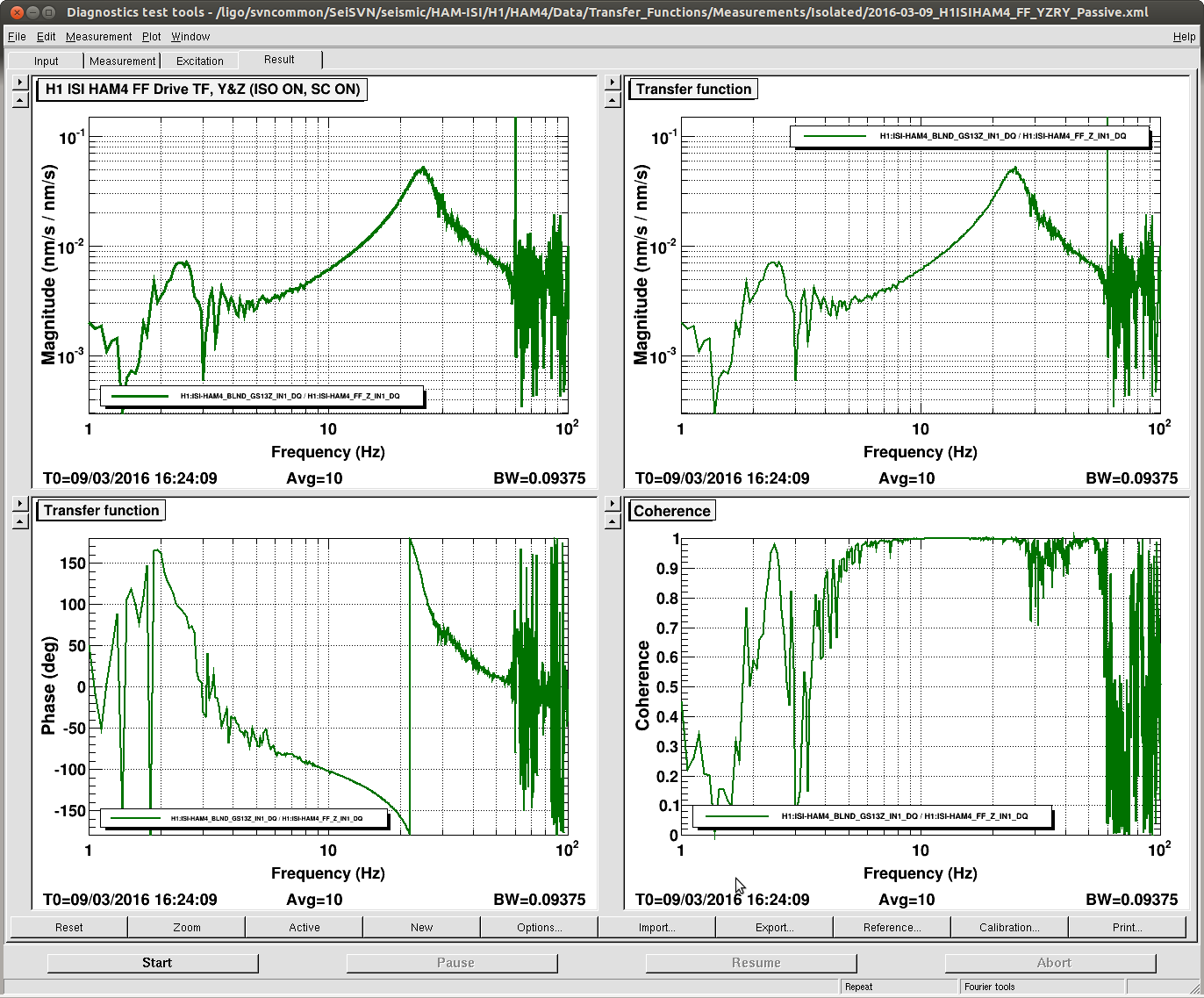
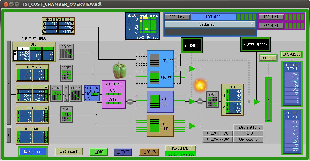
J. Kissel

While helping Nairwita debug the HAM-ISI noise budget model, I've found myself dreadfully ignorant of the HAM FF design which Jim has worked so hard. In this aLOG, I show and explain as much information as possible on the design of the filter, just that it (hopefully) becomes clear. This documents the design original elluded to in Jim's LHO aLOG 19292.

------------
Units.
Let's start at the overview screen, HAMISI_OVERVIEW.png. The filter banks marked as "FF" are our path, and notice that we have the option of using either the HEPI L4C or in-vac ST0 L4C sensors (both intertial sensors of the same time, just in different locations). For reasons to be discussed elsewhere, we've chose the ST0 L4Cs. Also recall that these L4Cs, like every ISI inertial sensor, has been *partially* calibrated, such that the high-frequency velocity response asymptotes to a flat 1 [nm/s], and rolls off at low-frequency as f^2, where the corner frequency for all instruments has been modified to be 1 [Hz], with a critically coupled Q of sqrt(2)/2. In short, we'll call these "velocity cts." The L4Cs are projected into the ISI's Cartesian basis and is piped into the FF filter where the green pepper is shown.
The output of the filter (indicated by the small explosion) is added into the feedback isolation loop path at the control point. That mean the output of the FF filter must be in the same units as the output of the feedback loop. Though we know the calibration from these "force counts" to N, we don't calibrate it in real-time, because we want to keep the control scaled to DAC counts, as per LIGO convention. 
That means the filter must have units of 
   (force ct) / (ST0 L4C velocity ct)
when installed into foton.

The Ideal Filter
Recall the point of feed-forward: to minimize the forces on the suspended stage. There are two mechanical forces on the stage:
    (1) Motion of ST0 couples through the mechanical plant and forces ST1 to displace. This transfer function is simply the stiffness of the springs.
    (2) Control forces from ST1 actuators displace ST1.
Using the notation from T1300645, 
    (1) = P^{'(0-1)} = "damped displacement plant" = fundemental units of [m/m] and 
    (2) = P^{'(1-1)} = "damped force plant" = fundamental units of [m/N].
In the absence in of any sensor corrected feedback control, that means the ideal filter, F^{FF} filters the control force such that it perfectly balances the input motion of the displacement plant
   F^{FF} P^{'(1-1)} + P^{'(0-1)} = 0
which we can manipulate to get an expression for the ideal filter:
   F^{FF} = - P^{'(0-1)} / P^{'(1-1)}
We immediately find was we expect -- the units of the above equation cancel out nicely to have the same units as a stiffness: [m/m] / [m/N] = [N/m]. The problem: this design process requires you to have a very good measurement (or model) of both P^{'(1-1)} and P^{'(0-1)}. While our actuators are strong enough to characterize the driven transfer function, P^{'(1-1)}, with oodles of coherence, we must rely on what SNR  we get get out of the residual ground motion to determine P^{'(0-1)} (i.e. coherence between our ST0 sensor and our on-board ST1 sensor)

Where / why we use Sensor Correction vs. Feed Forward
In reality, we have a sensor-corrected feedback system that's also trying to suppress the motion of ST1 at low frequency. That feedback loop alters the shape of the displacement and force plants in the region where the feedback loop gain is large. In this region, it reduces the coupling of the ST0 motion ot ST1 motion (i.e. P^{'(0-1)}) to essentially zero. Thus, we can only use feed-forward where the loop gain is small, and there remains enough coherence between ST0 and ST1 that P^{'(0-1)} can be measured well enough to design the ideal filter. In practice, that turns out to be between about 5-30 [Hz] for the HAMs.
Where the loop gain is large (below 5 [Hz]), we correct for excess coupling of ST0 at the error signal instead of the control signal, i.e. sensor correction. In a sense, this is also feed forward, (and in fact the filter design process is strikingly similar) but the injection point is ahead of the control filter and hence we distinguish it with different nomencalture. On advantage of sensor correction over feed-forward: the filter need not change if the feedback design changes (which is not true for feed forward, since both P^{'(0-1)} and P^{'(1-1)} are modified by the feedback loop suppression). One drawback of sensor correction: it relies on the feed-back loop gain. Feedback stability is quite restrictive at high frequency. Thus we use feed-foward to where-ever there is residual coherence in the P^{'(0-1)}.

The Measurements
We want to improve the isolation from 5-30 Hz, beyond what sensor-corrected feedback can do. So, all measurements are taken with the sensor correction and feed-back loops closed. For P^{'(1-1)}, one drives at the excitation point of the (at this point empty) feed-forward filter bank, and measures the response of ST1 (in the case of the HAM, we use the ST1 GS13 inertial sensors). In raw form, that means this "driven" TF measurement has units of
    P^{'(1-1)} = (ST1 GS13 velocity ct) / (ST1 force ct)
               = H1:ISI-HAM4_BLND_GS13Z_IN1_DQ / H1:ISI-HAM4_FF_Z_EXC
where the GS13s have been partially calibrated in the same manner as the L4Cs. For P^{'(0-1)}, with no drive, one measures the "passive" TF between the ST0 sensor and the ST1 sensor,
    P^{'(0-1)} = (ST1 GS13 velocity ct) / (ST0 L4C velocity ct).
               = H1:ISI-HAM4_BLND_GS13Z_IN1_DQ / H1:ISI-HAM4_FF_Z_IN1_DQ
Because the L4C and GS13s have both been calibrated in the same fashion, that means that the ratio of these transfer functions are already in exactly the right units for the ideal filter:
    F^{FF} = - P^{'(0-1)} / P^{'(1-1)} = (force ct) / (ST0 L4C velocity ct)
Though it's not needed for the filter design, if you want to model the platform motion in physical units, you've got to do a little unit juggling. From Eq. 9 in T1300645, the two terms concerning feed-forward are 
    z_{ST1}^{FF} =   P^{'(0-1)} / (1 - e G') z_{ST0}
                   + P^{'(1-1)} / (1 - e G') F^{FF} z_{ST0}
so if you which to input motion of z_{ST0} in displacement units, say [m], and you have a force plant in units of m / (force ct), then you'd better convert whatever filter you pull out of foton into units of [(force ct) / m], i.e. finish the calibration of the L4C by removing the displacement response,
    cal_m_p_ct_L4C.c   = (1/nm_p_m) * zpk([0 0 0],-2*pi*pair(1,45),prod(2*pi*pair(1,45))/(2*pi).^2);

The fit vs. cutoff-frequencies
On you have the measurement, and have computed the ratio of the two transfer functions, whereever their remains coherence in the measured P^{'(0-1)} measurement you want to fit that ratio as best you can. Outside of this region, you want to roll-off the feed-forward control as quickly as possible, while still maintaining as much fidelity of the in-band filter as possible. The pdf attachment reverse engineers Jim's design, with a whole bunch more labels, and shows the transfer function ratio cast into a few different units for comparison.

For a model of the predicted performance of the design -- we need Nairwita's work, since the performance depends on models of the feedback loop and force plant. Hopefull we'll get there soon!

Details:
You can run the script that generates the design study here:
/ligo/svncommon/SeiSVN/seismic/HAM-ISI/H1/HAM4/FilterDesign/FeedForward/designstudy_h1isiham4_ff_Z_20160310.m
as long as you update the following folders:
/ligo/svncommon/SeiSVN/seismic/HAM-ISI/H1/HAM4/Data/Transfer_Functions/Measurements/Isolated/  << to get all of the recently committed data
/ligo/svncommon/SeiSVN/seismic/Common/MatlabTools/ << to get a new function readdttexport.m