craig.cahillane@LIGO.ORG - posted 21:20, Wednesday 15 June 2016 - last comment - 23:59, Friday 17 June 2016(27765)
LHO Calibration Uncertainty - Now With Covariance
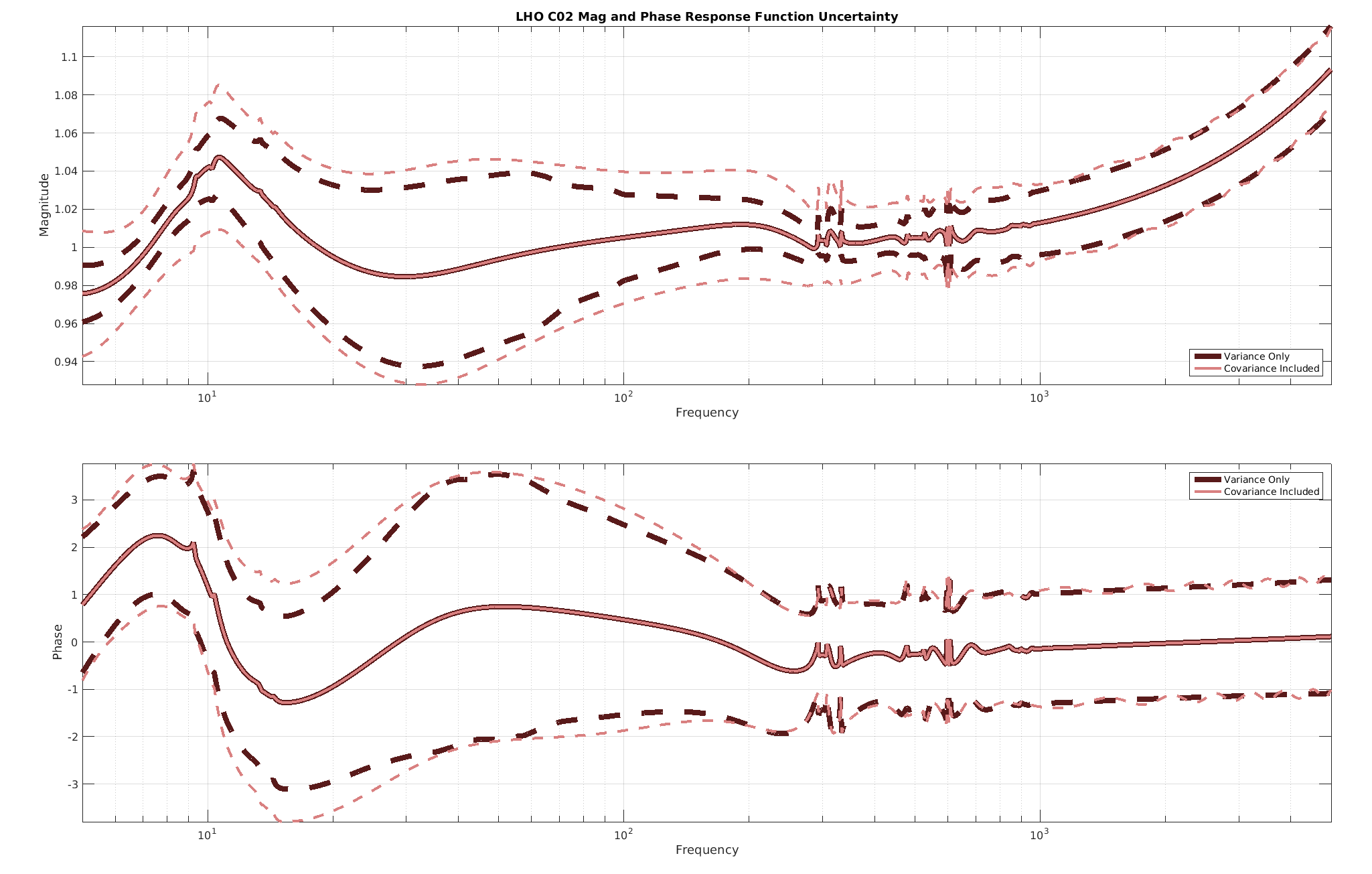
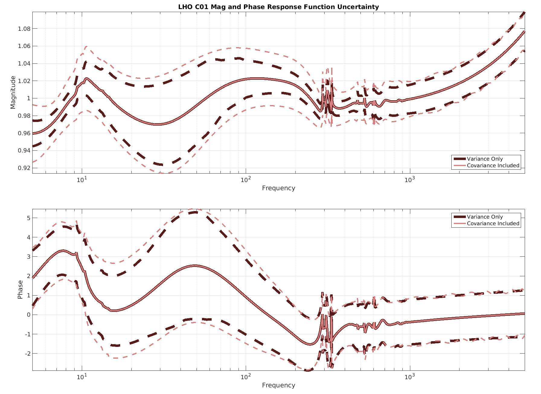
C. Cahillane I have revamped the uncertainty budget to include covariances between all stages of actuation and all time-dependent parameters. I computed each parameter's covariances in real and imaginary coordinates to provide a consistent basis. I then compiled an6 x 6Actuation Covariance MatrixC_A, a2 x 2Sensing Covariance MatrixC_S, and an8 x 8Kappa Covariance MatrixC_K. Then I compile them into a giant covariance matrixC:_ _ | C_A 0 0 | C = | 0 C_S 0 | |_ 0 0 C_K _|Then, I multiply by some conspicuous Jacobian vectorsJ(f)to get the final2 x 2uncertainty matrix σ_R^2(f):σ_R^2 = J * C * J'whereJlooks like:_ _ | d Re(R) d Im(R) | | --------- --------- .... | | d Re(p_i) d Re(p_i) | J(f) = | | | d Re(R) d Im(R) | | --------- --------- .... | |_d Im(p_i) d Im(p_i) _|(I was able to use complex differentiation and Cauchy-Riemann here to make the derivatives easier. Recall that R = 1/C + D*A. Now I can compute dR/dA = D and dR/dC = -1/C^2 to formJ(f), thanks to 200 year old mathematics) Finally, to make the uncertainties readable by humans, I divideσ_R^2(f)by|R(f)|^2, rotateσ_R^2(f)byangle(R(f))via a rotation matrix, and read off the square roots of the diagonal of the rotatedσ_R^2(f)to get the magnitude and phase uncertainties plotted below. I have plotted the uncertainty at GPSTime = 1135136350, the time of the Boxing Day Event. The plot shows an overall increase in magnitude uncertainty of about 1% at low frequency. Phase uncertainty increased by about 0.5 degrees at low frequency. The effects are more dramatic at Livingston. Check out LLO aLOG 26542.
Images attached to this report
Comments related to this report
C. Cahillane

I have reproduced the uncertainties including covariance for GW150914 for the calibration companion paper.  We will have to update the associated uncertainty calculation sections of the paper.
I have also attached two .txt files for the R_C01/R_C03 response comparison and the associated uncertainty.

Something I failed to emphasize above: Our uncertainties in the response function are now fully covariant... the plots I show of the magnitude and phase are only approximations to the true uncertainty.
I have looked at the 3D plots of the covariant ellipses, and it's a fairly good approximation in this case.
Images attached to this comment
Non-image files attached to this comment

C. Cahillane

I have attached and printed my relative covariance matrix.  Please see DCC T1600227 for an explanation of the relative covariance matrix.
Basically, the below is percentage covariances.


             Re(A_U)   Im(A_U)   Re(A_P)   Im(A_P)   Re(A_T)   Im(A_U)   Re(C_R)   Im(C_R)   Re(K_T)   Im(K_T)   Re(K_P)   Im(K_P)   Re(K_C)   Im(K_C)   Re(f_C)   Im(f_C)
Re(A_U)       0.0166    0.0083    0.0139    0.0079    0.0146    0.0067         0         0         0         0         0         0         0         0         0         0
Im(A_U)       0.0083    0.0209    0.0091    0.0169    0.0071    0.0178         0         0         0         0         0         0         0         0         0         0
Re(A_P)       0.0139    0.0091    0.0163    0.0052    0.0157    0.0066         0         0         0         0         0         0         0         0         0         0
Im(A_P)       0.0079    0.0169    0.0052    0.0181    0.0057    0.0156         0         0         0         0         0         0         0         0         0         0
Re(A_T)       0.0146    0.0071    0.0157    0.0057    0.0251    0.0047         0         0         0         0         0         0         0         0         0         0
Im(A_T)       0.0067    0.0178    0.0066    0.0156    0.0047    0.0187         0         0         0         0         0         0         0         0         0         0
Re(C_R)            0         0         0         0         0         0    0.0207    0.0079         0         0         0         0         0         0         0         0
Im(C_R)            0         0         0         0         0         0    0.0079    0.0208         0         0         0         0         0         0         0         0
Re(K_T)            0         0         0         0         0         0         0         0    0.0025   -0.0002    0.0019   -0.0018   -0.0004         0    0.0004         0
Im(K_T)            0         0         0         0         0         0         0         0   -0.0002    0.0025    0.0017    0.0019    0.0001         0    0.0001         0
Re(K_P)            0         0         0         0         0         0         0         0    0.0019    0.0017    0.0035   -0.0003    0.0002         0   -0.0003         0
Im(K_P)            0         0         0         0         0         0         0         0   -0.0018    0.0019   -0.0003    0.0035    0.0006         0   -0.0005         0
Re(K_C)            0         0         0         0         0         0         0         0   -0.0004    0.0001    0.0002    0.0006    0.0037         0   -0.0036         0
Im(K_C)            0         0         0         0         0         0         0         0         0         0         0         0         0         0         0         0
Re(f_C)            0         0         0         0         0         0         0         0    0.0004    0.0001   -0.0003   -0.0005   -0.0036         0    0.0054         0
Im(f_C)            0         0         0         0         0         0         0         0         0         0         0         0         0         0         0         0