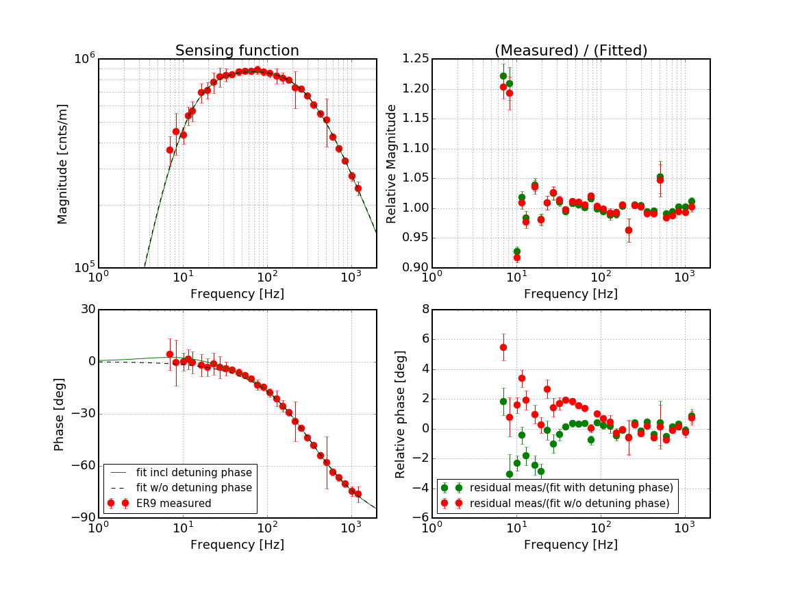
With the measured sensing function (28123) in hand, we did an MCMC-based numerical fitting for the sensing function (see E. Hall, T1500553).
The fitting results are
- Optical gain = 8.980393e+05 +/- 7.965381e+02 [cnts/m]
- Cavity pole = 3.294194e+02 +/- 5.626792e-01 [Hz]
- Time delay = 1.973719e+02 +/- 3.386483e-01 [usec]
- Spring frequency = 9.825078e+00 +/- 5.453538e-02 [Hz]
[New sensing function form]
As reported by Evan (27675), it seems that the extra roll off in the DARM response at low frequencies are due to an SRC detuning (or something equivalent). While such detuning should be suppressed by some control loop ideally, we decided to include the detuning-induced functional form in addition to the ordinary single-pole response. We use the following approximated form for the DARM response
S(f) = H / (1 + i f / fc ) * exp( -2 * pi * f * tau) * f^2/(f^2 + fs^2)
where H, fc, tau and fs are the optical gain, DARM cavity pole, time delay and spring frequency. Some details of the derivation will be reported later. Apparently, we now have an additional quantity (i.e., fs) to fit.
Note that since H1 seems to be in (unintentionally) an anti-spring detuning, fs should be a real number whereas it should be an imaginary number for a pro-spring case. Obviously, Q is set to infinity for simplicity.
[MCMC-based numerical fitting]
Following the work by Evan (T1500553), we adapted his code to include the spring frequency as well. In short, it is a Bayesian analysis to obtain posteriors for the parameters that we want to estimate. We gave a simple set of priors as follows for this particular analysis.
- 0 < H < infinity
- 0 < fc < infinity
- 0 < tau < infinity
- 0 < fs < infinity (real number)
The quad plot below shows the fitting result. The estimated parameters are obtained by taking the mean values of the resutling probability distribution. As usual, the two plots on the left hand side show a bode plot of the measured and fitted data. The two plots on the right hand side show the residual of the fit. As shown in the residuals, there are several points which are as big as 20% in magnitude and 6 deg in phase below 10 Hz. Otherwise, the residual data points seem to be within 10-ish % and 4 deg. The code is attached in pdf format.
EDIT: I am attaching the actual code as well.


A detailed derivation of the new functional form can be found at https://dcc.ligo.org/LIGO-T1600278
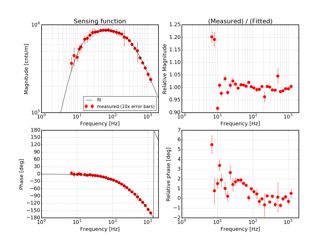
EvanG noticed that we have unintentionally included high frequency poles in the previous analysis (28157). So we made the same fitting for the data with all the high frequency poles removed.
Here are the fitting results for the latest data:
- Optical gain = 9.070764e+05 +/- 8.071988e+02 [cnts/m]
- Cavity pole = 3.287361e+02 +/- 5.692504e-01 [Hz]
- Time delay = 5.554816e+00 +/- 3.424867e-01 [usec]
- Spring frequency = 9.831483e+00 +/- 5.434934e-02 [Hz]
Since the bode plot looks very similar to the one posted above, I skip showing it here. Observe that the time delay is now smaller than it was because we now don't have the high frequency poles.
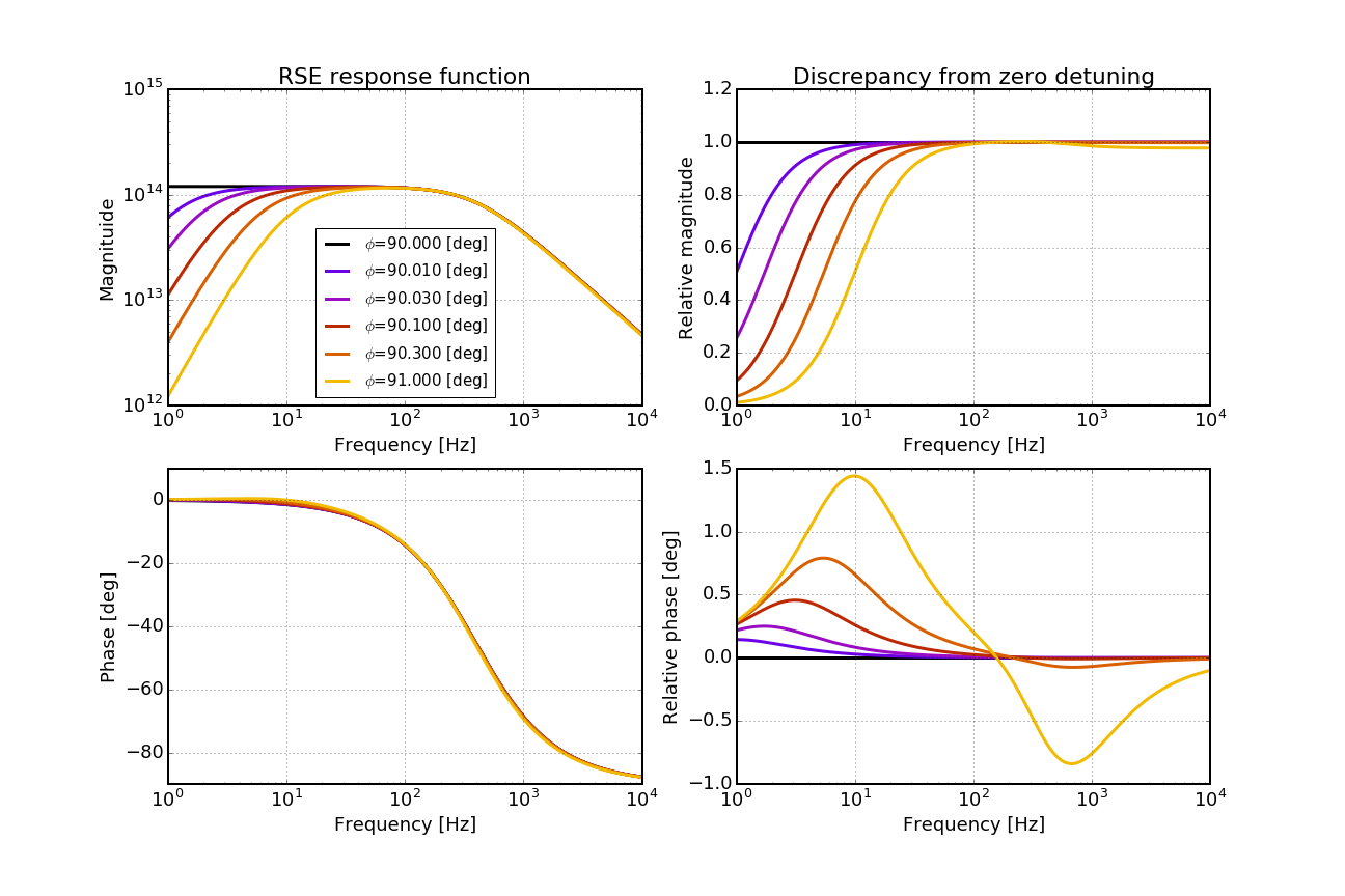
C. Cahillane, K. Izumi I have added in a new term to our sensing function fit, an optical spring Q factor to gain back phase information. From the functional form f^2/(f^2 + f_s^2) we only get a magnitude correction from detuning, but we also expect detuning to slightly affect phase in the sensing function response. This can be clearly seen in lower right subplot Figure 1 of this comment, where Kiwamu originally plotted the full RSE sensing function. Here we see that when we have 1 degree of detuning we also have +1.5 degree phase difference at 10 Hz when compared to the sensing function without detuning. In the phase residual plot in the original post you can see this phase loss in the actual ER9 sensing measurement. In order to try and gain back some of this phase information, we have added in an additional term to the detuning function:f^2 f^2 ----------- ===> ----------------------- f^2 + f_s^2 f^2 + f_s^2 - i*f*f_s/QThis adds another parameter to our fit, but lets us get back phase information lost to detuning. ********** Figure 2 shows Kiwamu's original fit parameters posted above in red alongside my new results in green. I argue that including the optical spring Q factor has improved the phase fit significantly. Quantitatively, here are the phase Χ-Square values:With Optical Spring Q Χ-Square = 85.104 Without Optical Spring Q Χ-Square = 819.28********** I have modified Kiwamu's SensingFunction.ipynb into a SensingFunctionSimulation.ipynb which fits to both phase and magnitude of the sensing function. SensingFunctionSimulation.ipynb is attached as a zipped file in this aLOG and is also in a Git repo called RadiationPressureDARM owned by Kiwamu. Fit parameters:Optical gain = 9.124805e+05 +/- 8.152381e+02 [cnts/m] Cavity pole = 3.234361e+02 +/- 5.545748e-01 [Hz] Time delay = 5.460838e+00 +/- 3.475198e-01 [usec] Spring frequency = 9.975837e+00 +/- 5.477828e-02 [Hz] Spring Inverse Q = 1.369124e-01 +/- 3.522990e-03(I choose to parametrize using inverse Q = Q^{-1} because Q^{-1} can be zero.)