After a lot of experimentation, I have found a way to improve the attenuation of frequencies below 9 Hz in the calibration by 1-2 orders of magnitude, without significantly increasing the computational cost or latency of the pipeline. Here is a list of what I've changed and what I've kept the same:
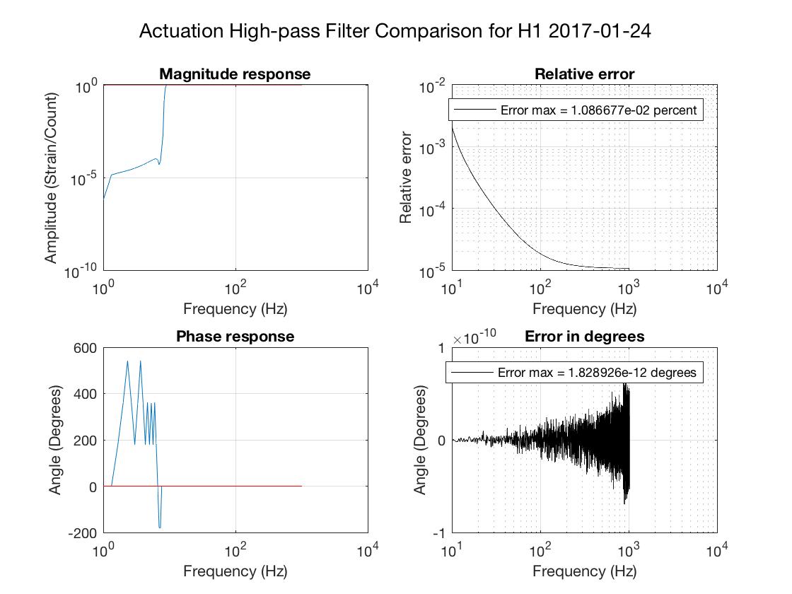
- In the actuation path, before the actuation filter, I have added a separate high-pass filter using Matlab's firls() function (documentation). firls() designs a linear-phase FIR filter that minimizes the weighted integrated squared error between the desired frequency response in specified intervals and the approximated response of the filter. The filter I've found most effective is designed to have a frequency response of 1 from 9 Hz to the Nyquist rate, and 0 from DC to 8 Hz. I found improvement when I weighted the stop band more heavily by a factor of 100. This filter was 2 seconds in length for the tests that I ran.
- I shortened the actuation filter itself from 6 seconds to 4 seconds. (The main reason we needed such a long filter before was to prevent spectral leakage, which is now taken care of by the previous high-pass filter.) It still contains half of a Hann window to the fourth power to roll off low frequencies, in order to further attenuate those frequencies. I found that this roll-off actually worked better than any version of least squares filter I tried in its place.
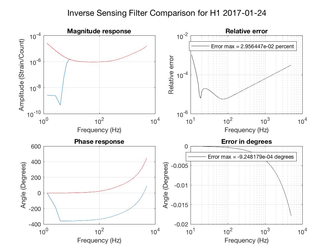
- In the inverse sensing filter, I replaced the half Hann window to the fourth power with Matlab's least squares filter using firls(). For some reason, this worked better in the inverse sensing filter than the Hann window stuff, even though it did not work better for the actuation. I designed this filter to have a frequency response of 0 from DC to 5 Hz (weighted by a factor of 100) and a frequency response of 1 from 9 Hz to the Nyquist rate. This is what seemed to produce the best results. I did not add a separate high-pass filter in the inverse sensing path, as it seemed unnecessary, and filtering at 16384 Hz gets expensive.
Of all the things I tried, this is what worked the best. Reasons I did not make this even better include:
- I haven't figured out a better way yet
- It is possible to do better with longer or more filters, but since we are doing this in the time domain with FIR filters, adding more filtering gets computationally expensive and adds latency. It is necessary to balance computational cost with quality, as we do not want the pipeline falling behind in low-latency or taking forever to produce offline data on the clusters.
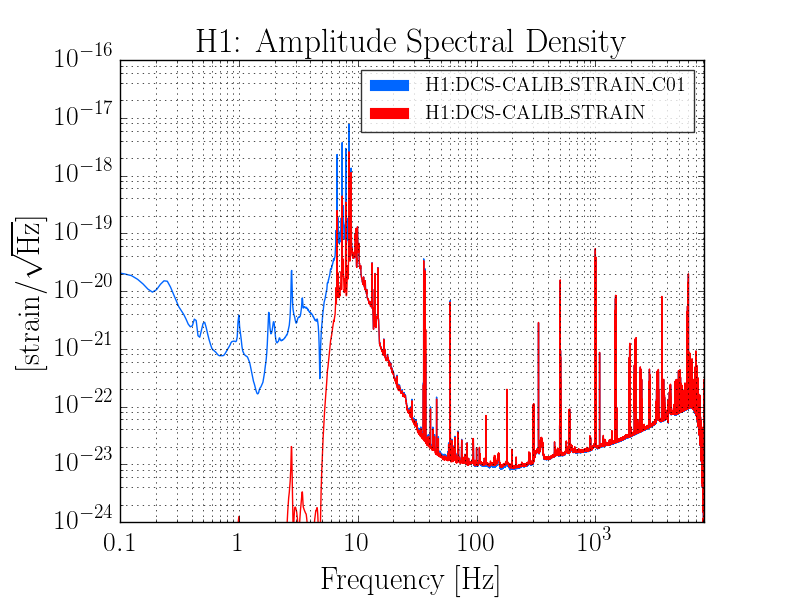
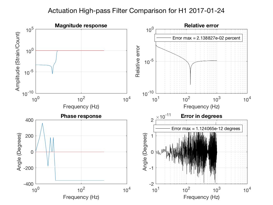
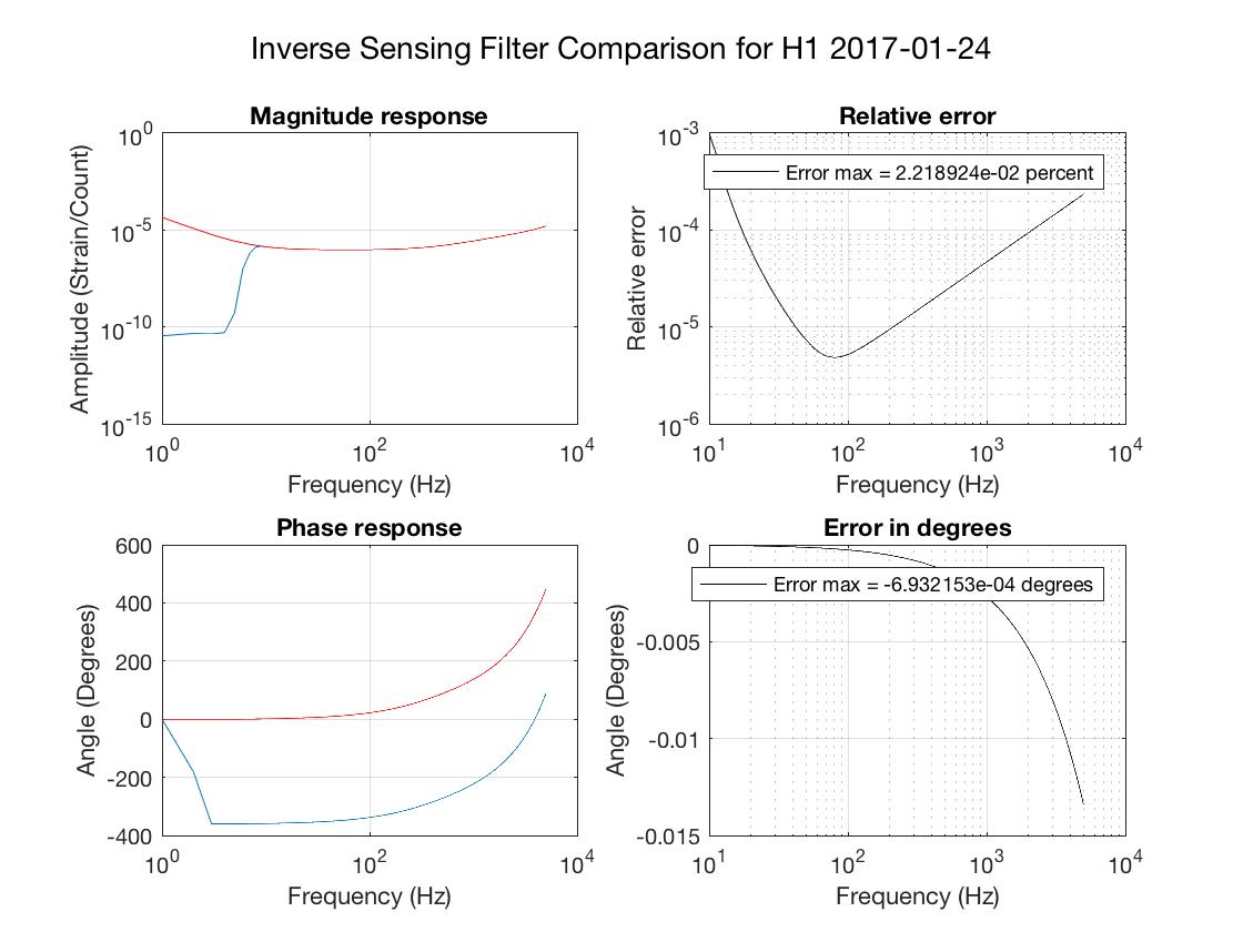
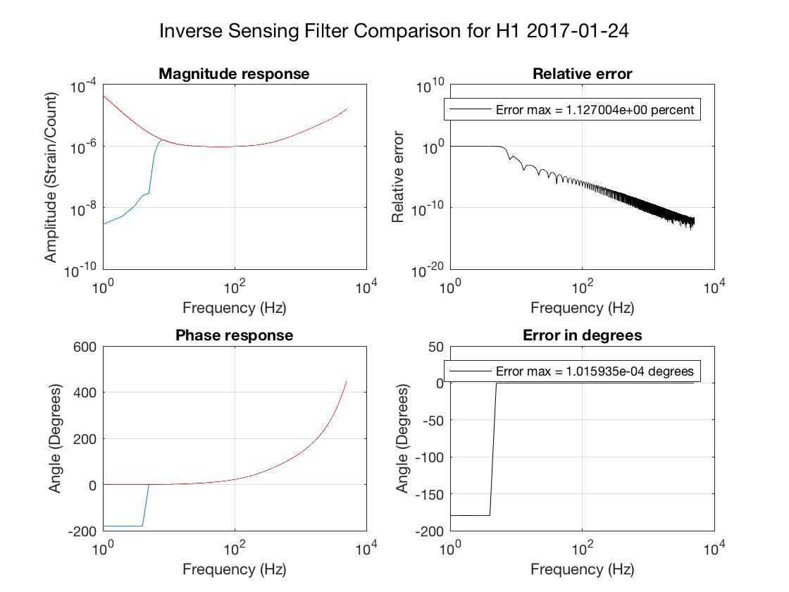
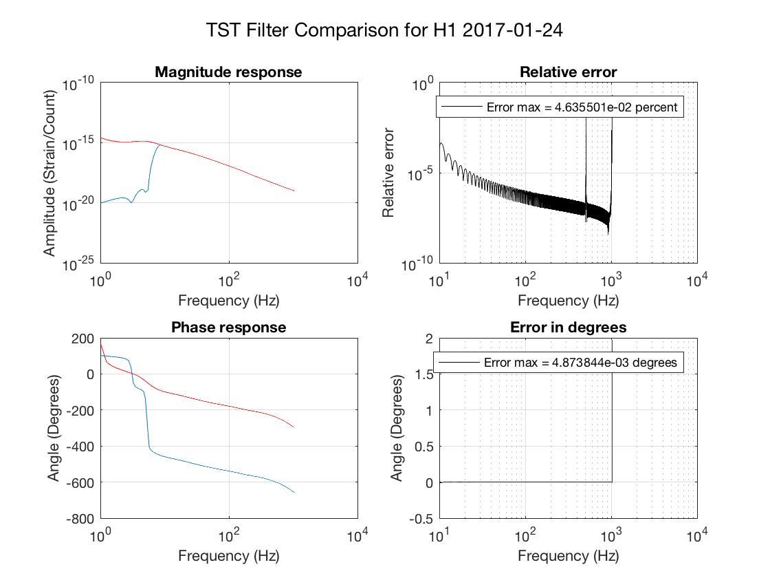
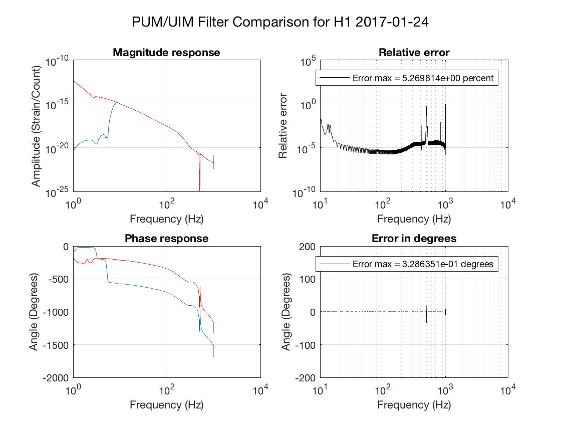
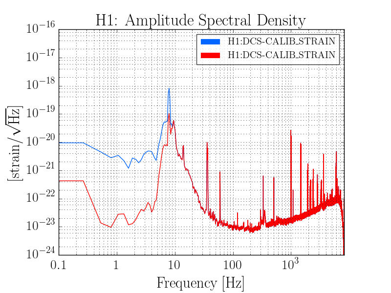
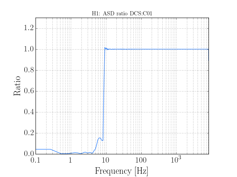
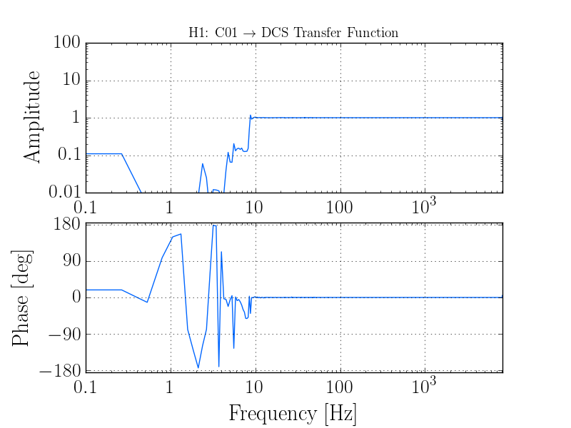
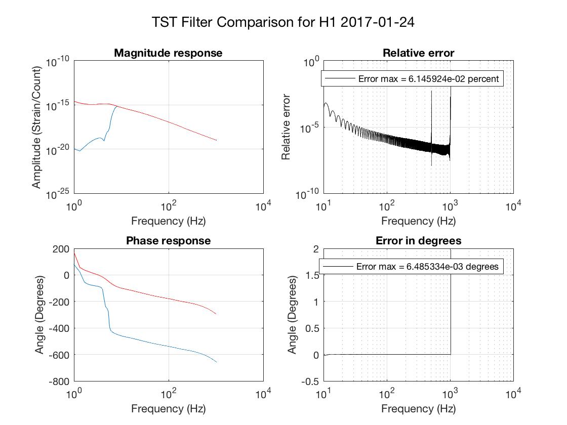
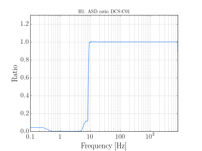
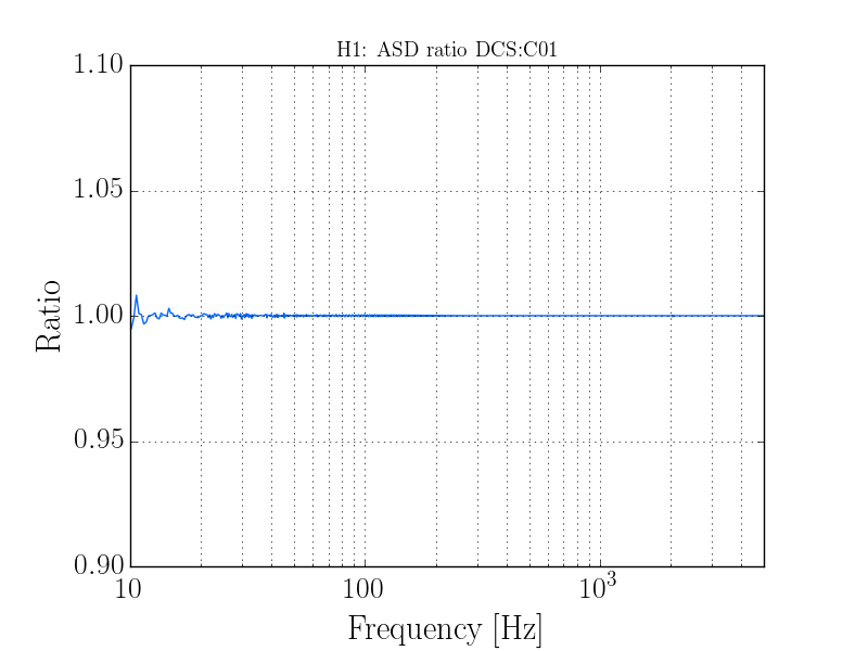
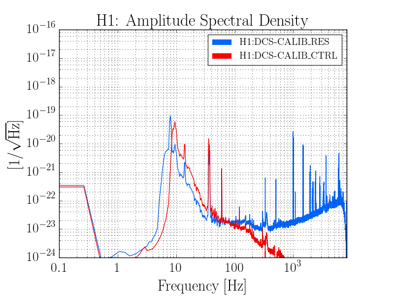
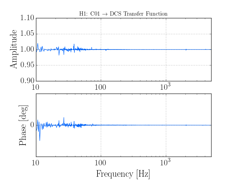
Several plots are attached to show the new features. The first 5 plots are the frequency responses and comparisons to the ideal models for each of the filters used. The last 3 plots are comparisons of C01 data with data produced using the new filters. The attenuation is better by about 1-2 orders of magnitude, and there is just a very small amount of ripple added below 20 Hz.
I have made some additional improvement in the high-pass filtering in the DCS filters. The additional changes I made were:
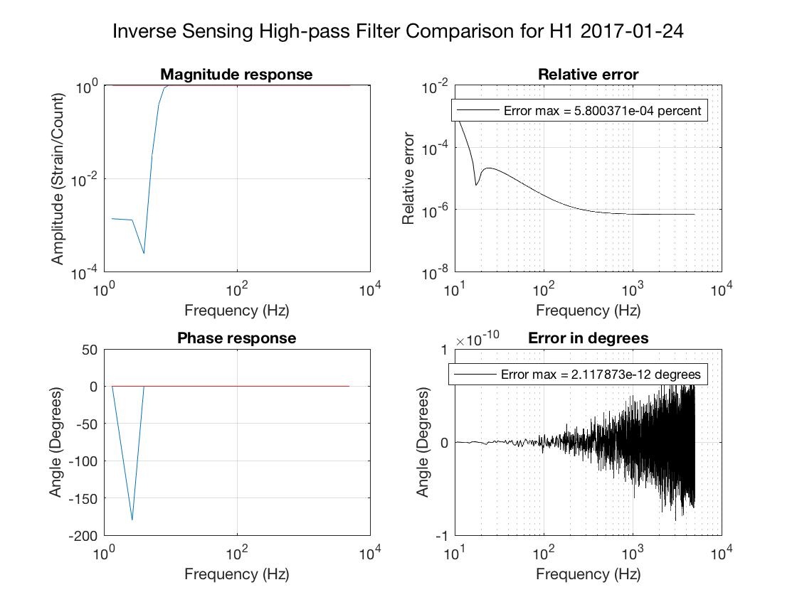
- Addition of a separate high-pass filter in the inverse sensing path before the inverse sensing filter. This also uses Matlab's least squares FIR filter, firls(). The cutoff frequency used is still 9 Hz, although I experimented with other cutoff frequencies. The filter is designed to have a response that drops to zero at 5 Hz and below. The length of this filer is currently set to 0.75 seconds.
- Shortened inverse sensing filter to 0.75 seconds. The inverse sensing filter was previously 1 second in length. Since DARM_ERR is filtered at 16 kHz, the total amount of filtering in this path (now increased from 1s to 1.5s) needs to be kept manageable.
- The actuation filter and the high-pass filter before it are now both 3 seconds in length.
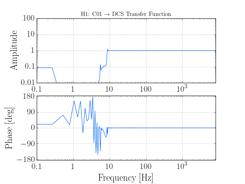
- In addition to the filers themselves, I have added code that writes the transfer functions corresponding to the combined effect of all filters applied to each path (inverse sensing and actuation). These are included in the filters files, so that they cannot be incorrectly paired with the wrong filters. In the DCS filters files, the names of these numpy arrays are invsens_filt_tf, tst_filt_tf, and pumuim_filt_tf. In the GDS filters files, the names are: res_corr_tf and ctrl_corr_tf.
- I also added a numpy array in the filters files that contains the filters' approximated response function. In both DCS and GDS filters files, this is called filters_response_function. In the GDS case, this gives only the portion of the response function that is applied by the GDS filters, not including the front end.
A similar set of plots is included, with several additions:
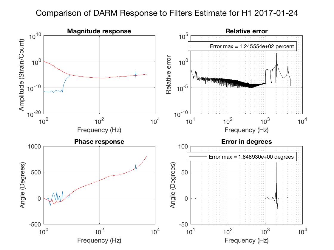
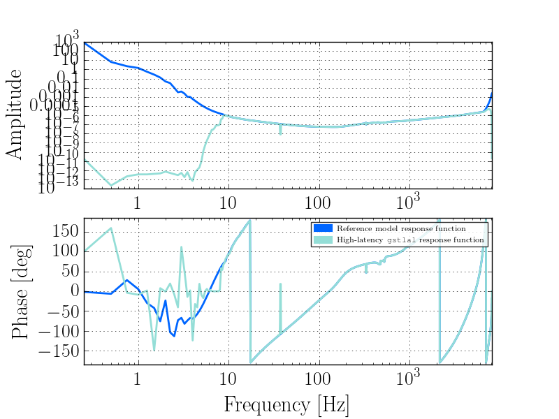
- I have implemented a new test of the filters that combines all the filters in the inverse sensing and actuation paths to show how well they approximate the model response function. A larger-than-expected error shows up above 1kHz where the contribution from the actuation filters drops to zero. I'm not yet sure why this is, but I'm not too concerned since it does not show up in the other response function plots, described next
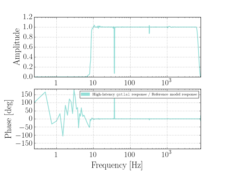
- I have also used a modified version of Maddie's response function plotting script to make plots of the response function as derived from the transfer function between DARM_ERR and DeltaL_free, and compare this to the model response function. (These are the last 3 files.) Errors from 10 Hz to 5 kHz look comparable to what they were before these changes. Note the small ~2% error just above 1kHz - this is due to the fact that the actuation is downsampled to 2 kHz in the gstlal calibration pipeline. At ~1kHz, the TST stage actuation still contributes a few percent to the total strain, leading to this ~2% error when it gets lost in downsampling. Notice also the few % error just above 10 Hz. There is a similar feature in the filters response function plot (described above), and in the PUM/UIM stage actuation filter.
It's also worthwhile to remind ourselves of the list of reasons why we wanted to improve this filter/what we wanted to improve:
- Search groups prefer aggressively high-passed data. Hopefully this is sufficient, as doing much better would significantly increase computational cost.
- Apparently the noise below 10 Hz has added to the difficulty of the data-cleaning effort. (?)
- It is ideal, when data goes public, that people don't find anything that could be mistaken for something significant below 10 Hz.
- There may sometimes be a need to model the high-pass filters in the gstlal calibration pipeline. Although common IIR filter representations like Butterworth, Chebyshev, and elliptic filters can be implemented as FIR filters, they are generally not the most effective. It takes a lot of taps to get a good filter; so it is more effective to use a different method (like minimizing the integrated squared error) to get the best filter we can for the lowest computational cost. Thus, the solution I propose to this problem is to use the transfer function that I have added into the filters files.
- There has been concern about the error around 10 Hz seen in the inverse sensing filter in these GDS filters and similar ones. GDS filters I've produced with the new high-pass filter do not show this behavior. However, as noted above the PUM/UIM stage filter does seem to introduce ~1% error just above 10 Hz. It is not clear whether this is related to high-pass filtering, but it is worth investigating.
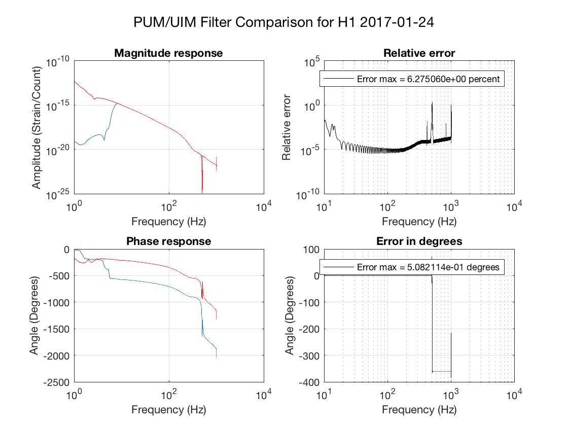
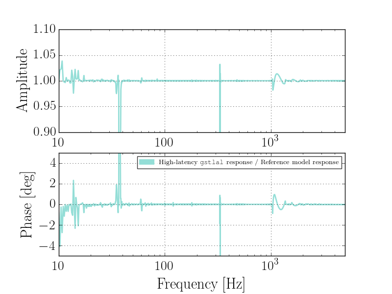
After further investigation, I've found that the the noted ~1% errors in the PUM/UIM stage filters just above 10 Hz are most likely due to notches in the actuation models at those frequencies, and do not seem to be affected by the high-pass filtering. One way to get rid of those errors is to remove the time-domain Tukey window from the filters. However, this generates a lot of noise in the spectrum due to the fact that the filters do not fall off smoothly.
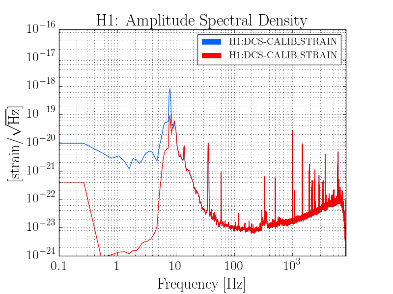
I also found that the "shelf" seen at low frequency in the ASDs (the noise from DC to ~0.25 Hz) may be an artifact of the relatively low frequency resolution (I used 3-second FFTs, so 0.33 Hz resolution) in the calculation of the ASDs. I have produced another ASD from the same data using 64-second FFTs averaged over 12 hours. The "shelf" is not seen here. I also investigated the possibility that this is a DC component (in which case it would still be present in the new ASD I plotted, but not shown due to the higher resolution). I added a feature the the gstlal calibration pipeline that allows the option to remove a DC component from the data before filtering it. The method is to simply downsample the input data to 16 Hz (with high-quality anti-aliasing), take a running average of 16 seconds, and then upsample (with high-quality anti-imaging) and subtract the result from the input data. This can be done with zero latency by shifting the timestamps becuase the phase of a DC component is zero regardless of timestamp shifts. The result of removing the DC component before filtering was indistinguishable from not removing it, implying that this is not a DC component.
The attached plot shows a high-resolution spectrum comparison of C01 data to data produced using the new high-pass filters. There appears to be a line present around 3 Hz. The small differences between C01 and the new DCS data above 10 Hz are due to the fact that the kappas were not applied in producing the new data (I used the same data to produce the comparison to the modeled response function, which requires not applying the kappas).