I created an improved script to analyze the Optical Spectrum Analyzer data [the script can be found in /opt/rtcds/userapps/release/isc/h1/scripts/osa.py]
In summary:
- the script grabs the OSA data and performs two kind of peak extraction
- simply look for the upper and lower 45 MHz sidebands and integrate the power around them. Then look for the highest peak around the mid point of the two sidebands, call it the carrier, and integrate all the power.
- using the 45MHz sidebands, calibrate the OSA scan in units of modulation frequency, and then fit peaks at +/- 45 MHz, +/- 9 MHz and 0 MHz, to extract also the 9 MHz sidebands.
- the script can save the processed peak amplitudes to a file, with the GPS time
- the script can also save a second-long average of the OSA scan to a folder, for future post-processing
- the script can read the saved scans and reprocess them offline
gabriele.vajente@zotws2:~/$ /opt/rtcds/userapps/release/isc/h1/scripts/osa.py -h
usage: osa.py [-h] [-f FILENAME] [-t TIME] [-o OUTPUT] [-r REPROCESS]
optional arguments:
-h, --help show this help message and exit
-f FILENAME, --filename FILENAME
File where the time series of sideband and carrier
powers will be saved
-t TIME, --time TIME Duration of plotting window in seconds
-o OUTPUT, --output OUTPUT
Name of a folder where the average OSA scans will be
saved
-r REPROCESS, --reprocess REPROCESS
Reprocess scans from a folder, and save a
reprocessed.txt file in thereWhen running online, the script produces a plot like the one below, taken during a power up.
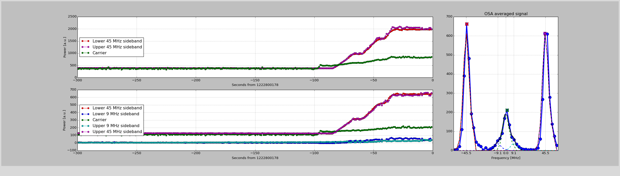
The two left panels contains the time traces of the peak powers. The top panel shows the "simple" peak reconstruction as explained above (simply identify the 45MHz peaks, integrate their power, find the largest peak in the middle and integrate its power). The bottom panel instead shows the more "advanced" reconstruction of the 45 MHz, 9 MHz and carrier peaks, by fitting peaks at the correct frequencies.
The right panel shows the latest averaged scan (blue dots and trace) plus some fitting and peak identification traces: the red, green and magenta X show the peaks used for the "simple" reconstruction (time traces in the top left panel); the dashed curves show the individual fits to the sidebands and carrier peaks (time traces in the bottom left panel); the black trace shows the sum of all fitted sideband and carrier peaks.
The 9MHz sidebands are very close to the carrier peak. When at low power, it's hard to resolve them. Even at 10W, they barely make bumps on the side of the carrier peak. So their power measurement has a quite large uncertainty and should be taken with care.