Using the noise injections described in 44868, with the LSC feedforward off, I computed the optical response (sensing matrix) of the LSC error signals, which is the calibrate response in cts/um of each of the XXXX_IN1 signals. I could get a good measurements for most of the elements of the 4x4 matrix, at frequencies between ~10 Hz and ~200 Hz.
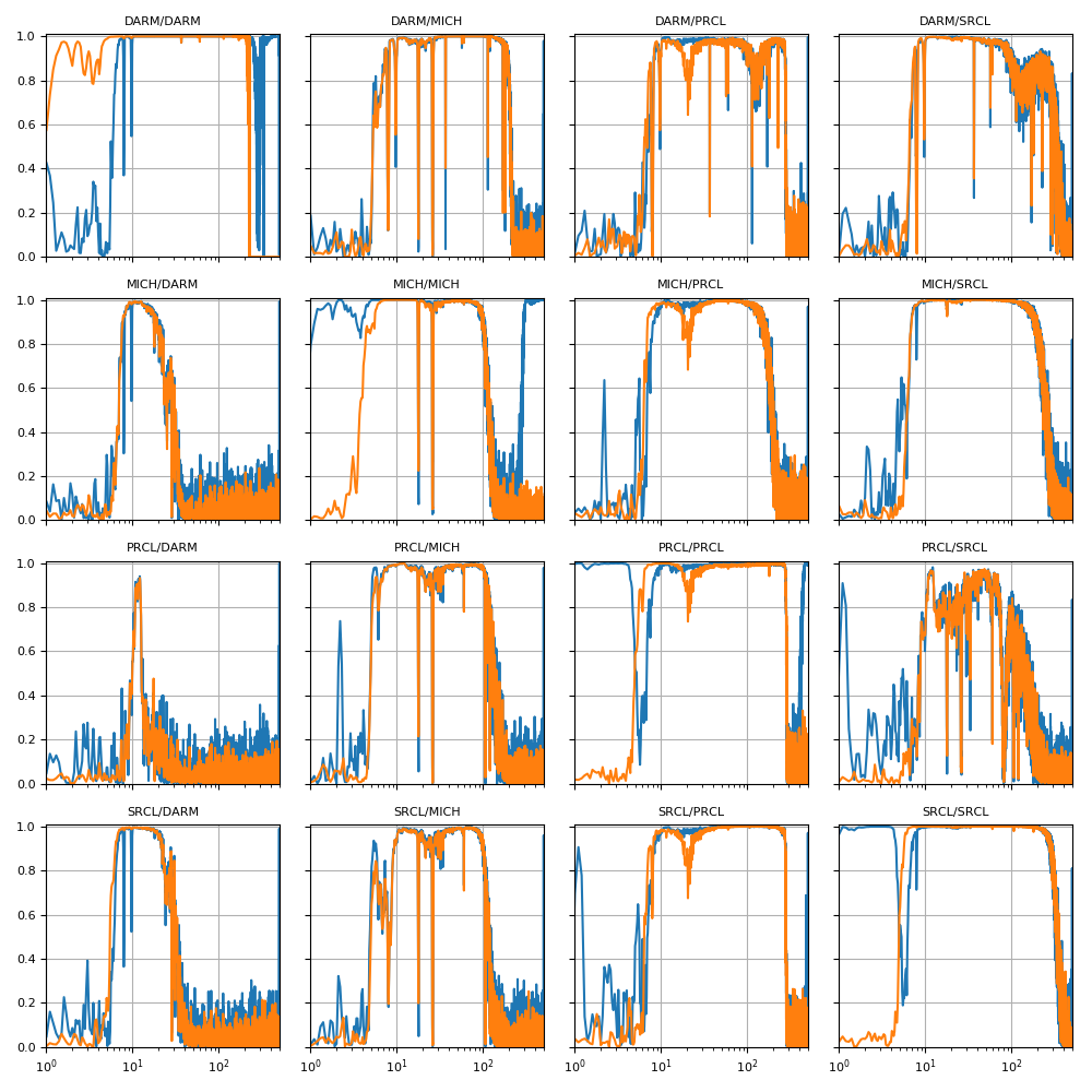
First of all, here is the coherence and transfer function matrices for the measurements. What is shown here is:
(left) coherence between injected excitation and input signals in orange (for example DARM_IN1 / DARM_EXC) and between the LSC control output and the LSC inputs in blue (for example DARM_OUT / DARM_EXC). This coherence matrix gives you a idea of where the measurements are good;
(right) transfer functions between the LSC output and the LSC input, in blue for all frequencies, in orange where there is coherence above 0.7.
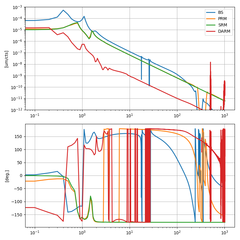
To extract the optical gain matrix (the response of input signals to actual d.o.f. motions in microns), I needed a model of the suspension response. Being lazy, I decided to cheat and use the model already implemented in the CAL system: for BS, PRM and SRM I copied the suspension model for M1, M2 and M3 stages from the CAL system. For DARM, since the model is much more complicated, I simply measured the transfer function between H1:CAL-DARM_CTRL_DBL_DQ and H1:CAL-DELTAL_CTRL_DBL_DQ while locked. To avoid numerical issues, I had to use 1000s long FFTs. As a by-product of this analysis, I updated the filters used in the CAL model, to match what is actually being used now in the SUS models (see 44891). Here are the suspension responses in microns over cts (at the ISC input point):
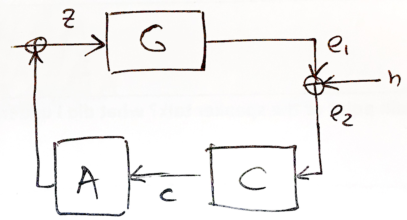
The transfer function matrix is measured between the LSC output and the LSC input. Where the signals are dominated by the injected excitation, the measurement is simply the product of the optical matrix (G) and the actuation matrix (A). In the scheme below, C is the control filter matrix. Here it is important to note that our MICH actuation is actually going only to the BS, so it is really a mixture of MICH, PRCL and SRCL actuation.
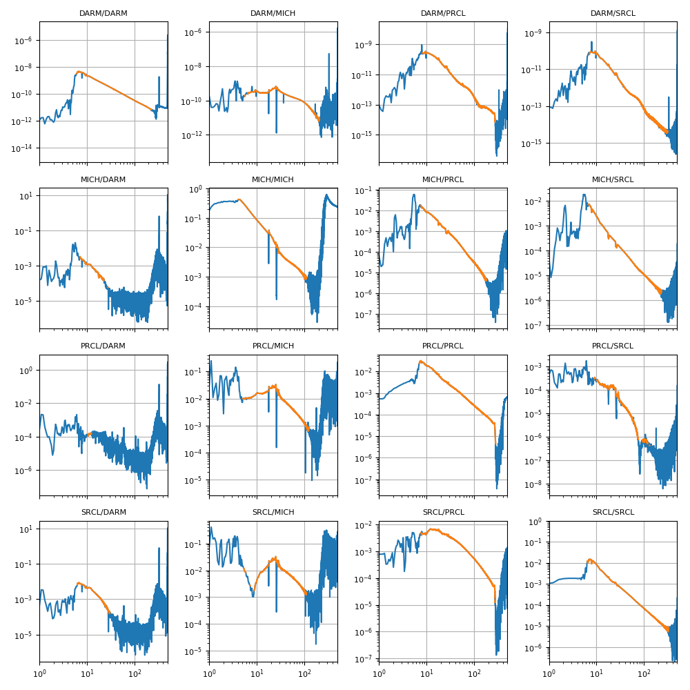
The resulting sensing matrix is shown below, in cts/um.
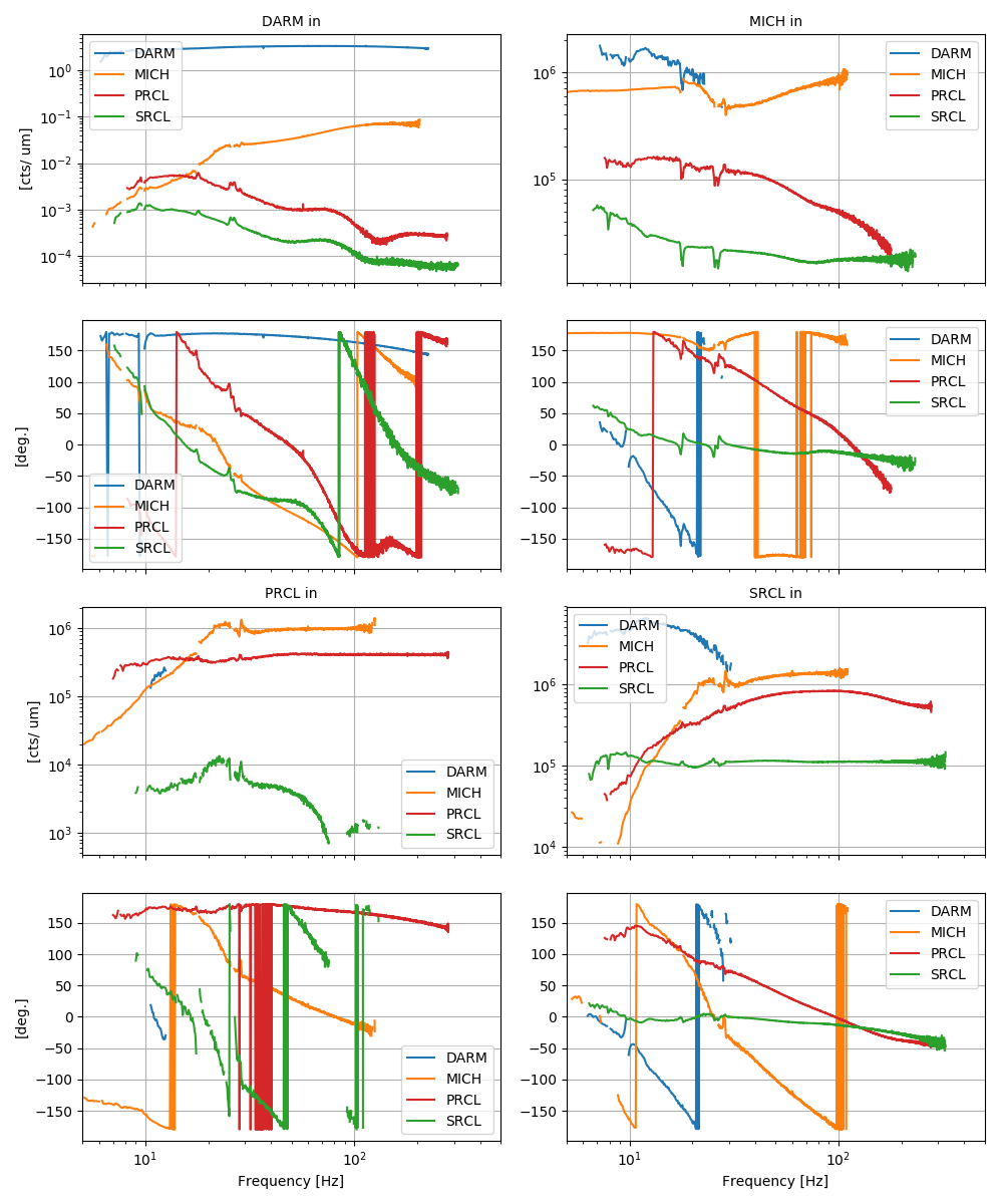
Each panel shows the response (magnitude and phase) of one of the LSC error signal, as noted in the title. For each panel, each trace then is the contribution coming from one of the LSC d.o.f.s (noted in the legend).
The response of each error signal to the "main" degree of freedom is more or less as expected. I updated the CAL error signal calibration with the new numbers, and as noted in 44891 the differences are small.
Some things are as expected, some other are a bit surprising. For example:
- there is a very large coupling of MICH to PRCL and SRCL, to the point that MICH is the dominant signal there. Since out MICH is actually BS, we expect some coupling into PRCL and SRCL, but not a dominant contribution like in this case.
- the DARM contribution to all signals is quite large at low frequency, which is something I don't quite understand yet
- MICH repsonse is not as flat as one would expect. Maybe this is due to the cross-coupling to PRCL and SRCL.
Finally, the plot below shows a table of the open loop gains, computed at the displacement point, i.e. each panel show DOF_Z_before_noise / DOF_Z_after_noise. The diagonal terms are as expected the open loop gains of the loops. The off-diagonal terms should be small in a ideally diagonalized MIMO system. However, here it's clear that some of the contributions are quite large: the MICH/PRCL/SRCL matrix has quite large elements at low frequencies (below 20-30 Hz). Also the DARM contribution to some d.o.f.s is much larger than expected. I am not sure how to interpreter this.
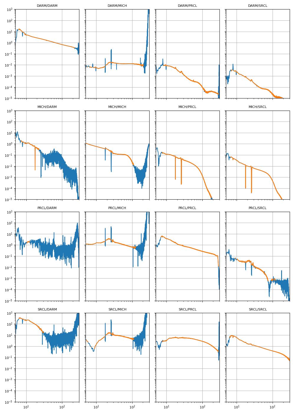
As before, blue are all points, but orange are only the frequencies with coherence.