Summary

This is an update on my previous activity on the characterization and subtraction of the non stationary SRCL coupling. See 45403 and 45508 for an introduction to the problem and methodology. In those elogs I developed a frequency domain method to compute how ASC signals modulated the SRCL to DARM noise coupling. In addition to that technique, I now have a parametric algorithm, that is capable of directly finding the optimal parameters to be used to implement stable and realizable time domain subtraction filters. For those of you familiar with Wiener filtering, this technique can be viewed as an IIR Wiener filter that also includes noise coupling modulations. More details on this technique are available in the DCC T1800525.

Here, instead of using the same data that I analyzed for 45403 and 45508, I used Rana's noise injection (45803 and 45792). In 45803 I derived the optimal filter to subtract the stationary coupling from SRCL_IN to CAL-DELTAL_EXTERNAL, using data without any noise injection. Here instead I used 150 seconds of data starting at GPS 1228458231 while there was a SRCL noise injection. My algorithm was tuned to use 16th order coupling transfer functions, and all ASC input signals as modulation sources.

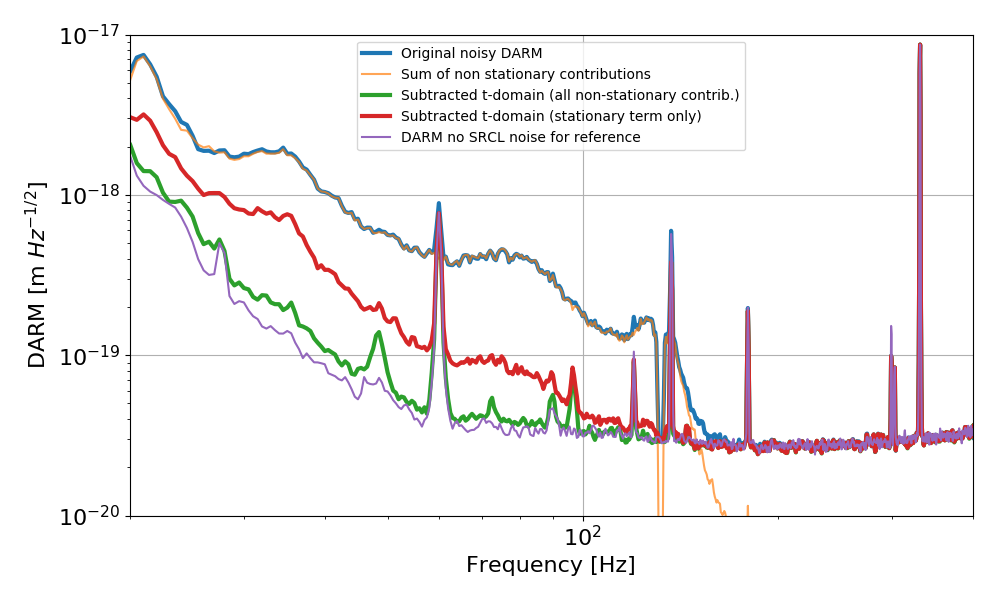
First of all, the money plot. The blue trace is the CAL-DELTAL spectrum during the SRCL noise injection, while the purple line is a reference from a few minutes before that, when there was no injection. The red trace is the best subtraction we can obtain using only the static, linear transfer function from SRCL_OUT to CAL-DELTAL. The green trace instead is the level of subtraction we can achieve including all non-stationary contributions. It is quite close to the DARM noise floor. The SRCL noise coupling reduction we obtain here is somewhat lower than what I could obtain in 45508: my guess is that is due to the fact that the SRCL injection was not as strong as the one that I did, so there was not enough SNR to extract even lower modulated contributions.

Nevertheless, by including the non-stationary contribution we can gain a factor of a few subtraction at all frequencies.

More details below

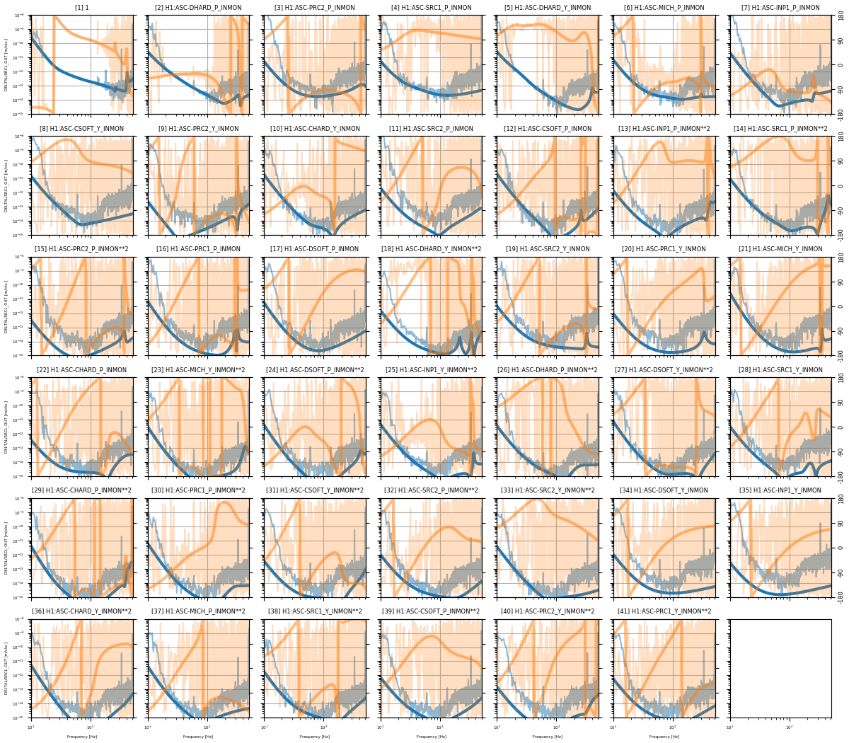
The plot below shows the reconstructed coupling transfer functions. Each panel correspond to one noise source, i.e. SRCL_OUT multiplied by the ASC signal in the title (where '1' means just a constant signal equal to one, that is, the stationary channel). The noisy traces in the background are the frequency domain direct solutions, while the solid smooth traces are the 16th order transfer functions obtained with a special s-domain transfer function parametrization that enforces the pole stability (and causality). The blue traces are the absolute values (refer to the left y axis) and the orange traces are the phases (refer to the right y axis).

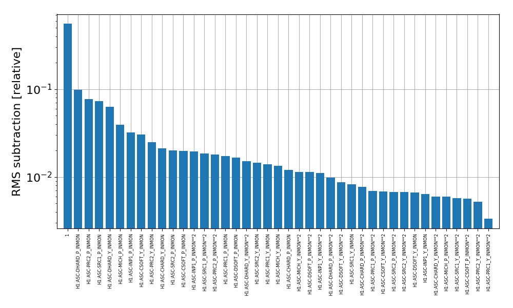
The contributions are sorted based on a ranking which computed what is the contribution of each modulation to the total noise subtraction, integrated between 10 and 400 Hz in this case. The numerical ranking of each ASC channel is reported below

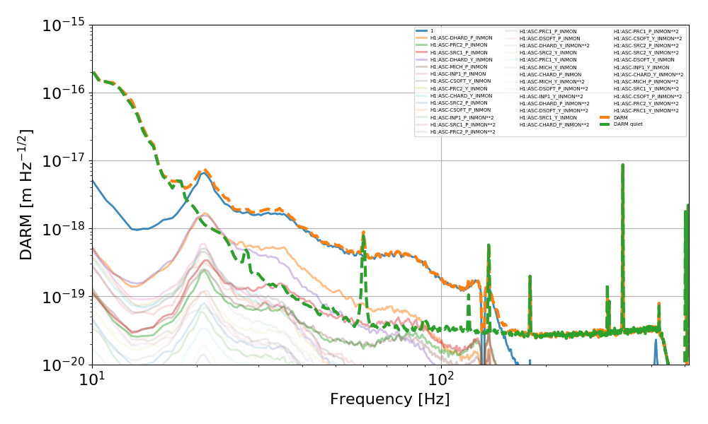
Another way to look at this is to plot each contribution in a spectrum of DARM, as below: