An attempt at a model of scattered light

My goal was to see if we can build a consistent model of the scattered light noise coming from OMC ASC motion, based on Georgia's injections (47446). Hopefully the A2L improvement described by Jenne (47488) will mitigate the problem.

For future reference, below the times of 0.5 Hz line injection:

'ANG_X': [1236416153, 1236416985, 1236416435, 1236416612],
'ANG_Y': [1236398014, 1236398260],
'POS_X': [1236398867, 1236398529],
'POS_Y': [1236399517, 1236399737],
'quiet': [1236422949]

The model is the same I used in 47423, but this time I used a linear combination of all four OMC ASC signals ('H1:OMC-ASC_ANG_X_INMON', 'H1:OMC-ASC_ANG_Y_INMON', 'H1:OMC-ASC_POS_X_INMON', 'H1:OMC-ASC_POS_Y_INMON') as the witness for the scatterer motion. So we have four k coefficients and two f coefficients:

where x_i are the OMC signals, "band-passed" ad 0.5 Hz as described in 47423. 

I considered two possible approaches to the fit of the parameter model:

1. treat every injection separately, and fit the optimal parameters independently for each of them
2. fit the same parameters to all injections simultaneously

In both cases I did not include the quiet time in the fit.

Fit each injection separately

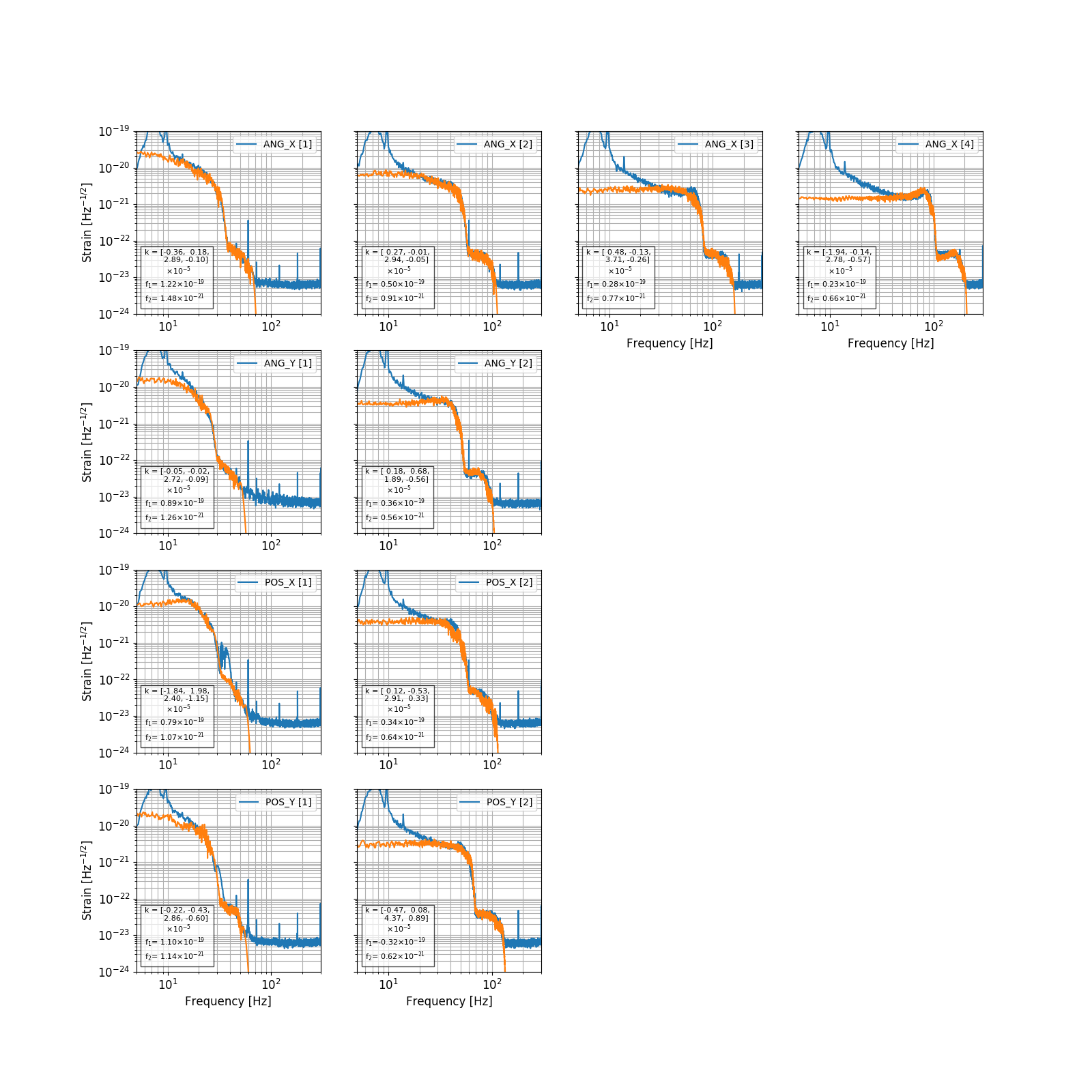
The plot below shows the best fit of the scattered light model above for each injection separately. You can see that the model fits all injections quite well, but the optimal parameter in each case are quite different. In all cases it seems the largest contribution to building the witness channel comes from H1:OMC-ASC_POS_X_INMON. But the value of the k coefficient that converts the witness to scatterer motion varies a lot, as well as the coupling coefficients f_1 and f_2. The blue curve is DARM, the orange curve is the modeled scattered light noise. The parameters for each fit are listed in the box in each plot.

 

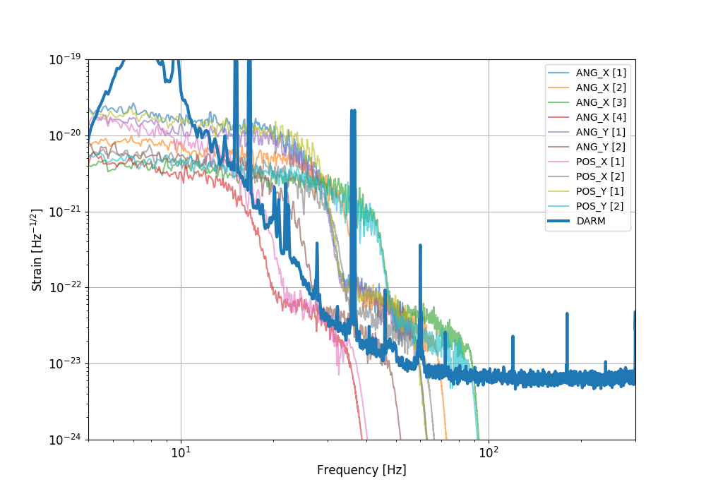
Applying each of these fit parameters to the quiet period gives us a busy plot, that shows how most of the fits overestimate the noise in the quiet case.

 

Fitting all injections all together

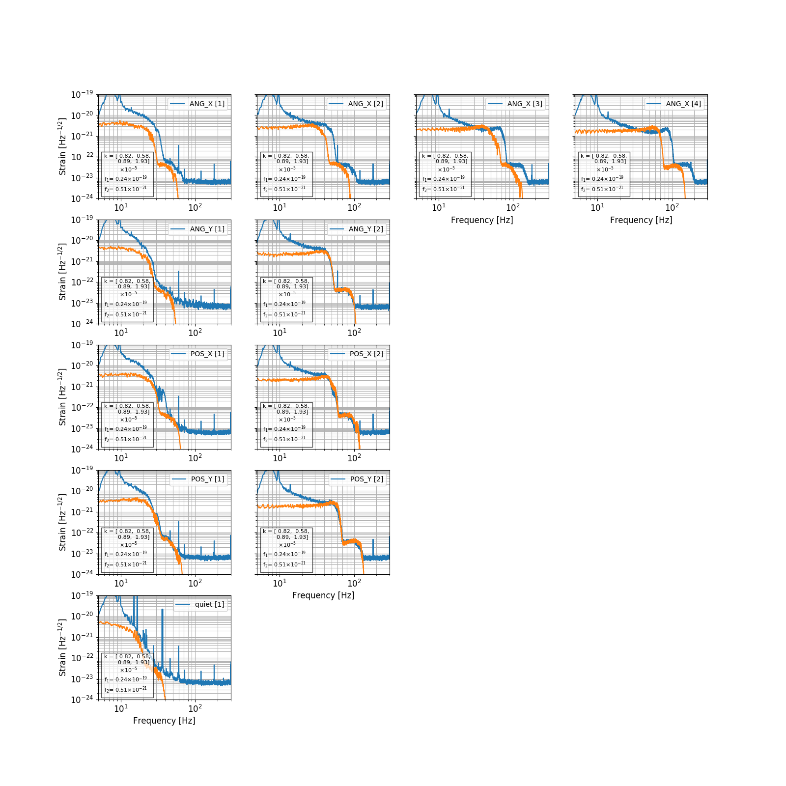
Assuming that the same scattering physics applies to all the injections (even if they're along different directions and separated by hours), we can force the fit to use the same parameters for all injections. The results are shown below. Now the very last plot shows the projection for the quiet time using the best parameters. The POS injections are fit well, while the ANG injections aren't that good. At least with these parameters (shown in the plot) the quiet time projection isn't overestimated anymore. 

 

I also tried other approaches, like allowing the per-filtering of the OMC signals to be a parameter (both as a band-pass Butterworth or a generic second order stage), without any more success than the global fit above.

In any case, it seems safe to assume that in normal operation, scattered light from OMC ASC motion is close to the measured sensitivity.

Some thoughts on why the same model parameters don't work for all injections

1. the up-conversion physics might be different from simple beam scattering: for example there can be a modulation that comes from clipping
2. maybe the OMC ASC sensors are good only at some frequencies, or we need to account for frequency dependent pre-shaping, for example due to the ASC loops
3. we haven't quite found the right witness sensor: maybe when we shake the OMC ASC we are inducing a motion of the real thing, but we don't have a good measurement of what that is