J. Kissel, L. Sun

While Lilli and Joe were tackling signing inside the CAL group's measurement *fitting* scripts, I was slogging away at trying to fight for measuring lower frequency data points to resolve the low-frequency side of the pro-spring detuned sensing function to better constrain the fit.

I was successful in measuring the full features of the detuning, but *answer* for the phase doesn't make sense.

I attach three plots:
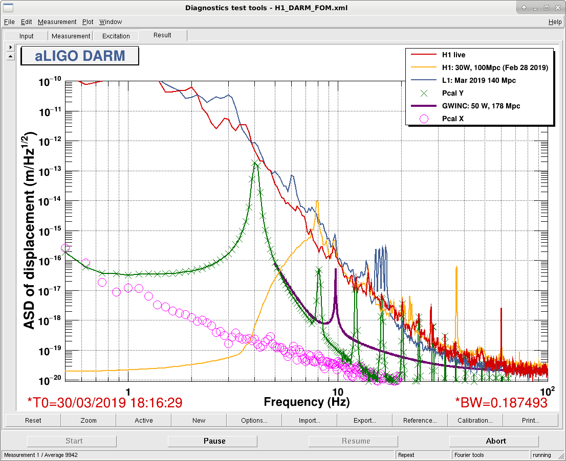
    (1) 2019-03-30_H1_DELTAL_EXTERNAL_vs_PCAL_0p5Hzto100Hz.png 
        We need to drive PCAL at it's maximum in order to get any semblance of SNR / coherence. The ASD of DELTAL external vs. PCAL during the lowest frequency parts of the measurement reveals how many integration cycles I needed in order to get any semblance of SNR [nCycles was 150]. You may notice the RX PD is exposing that the optical follower servo is driving significant amounts of harmonics of power on to the test mass, and be worried that this is spoiling the fidelity of the linear transfer function. Do not fear: we used the PCAL's RX PD as our reference, not the PCAL excitation, so while we may have less power in the fundamental than we request, it is still this power *at* the fundamental that we use as reference in the linear transfer function to DARM.

    (2) 2019-03-31_H1_sensingFunction_mcmcModel_vs_measurement.pdf 
        The output of the MCMC fit on this new data, to show the current status of our canned technology of fitting this data, and

    (3) 2019-03-31_H1_sensingFunction_modeldemos_vs_data.pdf
        An extension of my demonstrative plot yesterday comparing a pro-, anti- and bogus- spring zpk-decomposable transfer functions, but now includes the physical equation for the detuned sensing function. 
None of the models explain the phase of the measured sensing function well.


For the physical model, I dug back in to Evan Hall's thesis P1600295,, gathering material from Sections 2.3, 5.2, and Appendix D, and guided further by his distillation G1601599 plus the Craig / Kiwamu note T1600278.

After a hefty amount of algebra, Evan boils down Equation (3.83) in Rob Ward's thesis, P1000018, whom boiled it down from Eq. (2.20) of Buonanno & Chen (2001) arXiv:gr-qc/0102012, to arrive at his Equation (5.2) that describes the response in terms of poles and zeros,

    dP                          1 + i f / z
   ---- = g * ----------------------------------------------------    Eq. (5.2)
    dL-       [ 1 + i f / ( |p| Q ) - f^2 / |p|^2 ] +/- xi^2 / f^2

where

dP / dL- = the interferometer response (at the AS port) to DARM
       g = the optical gain (in this case in [(Watts at AS port) / (meter of differential DARM)])
       p = a complex coupled-cavity pole frequency, composed of the arm cavity pole(s) frequency and again, a term related to SRM reflectivity (in amplitude, so sqrt(0.32)) and SRC detuning phase (in radians)
       z = a real coupled-cavity zero frequency, composed of the arm cavity pole(s) frequency and a term related to the SRC detuning phase, and this time the readout homodyne angle
       Q = the quality factor of the coupled cavity pole frequency, valued determinisitcally by the value of p
    xi^2 = the (positive "pro" or negative "anti") square SRC detuned spring pole frequency, depending on lots of things including
               - the arm cavity pole(s), laser, and gravitational wave frequencies
               - the laser power on the beam splitter,
               - the length of the arms,
               - the mass of the test masses,
               - the SRM reflectivity, and
               - the SRC detuning phase


Now -- he discusses in words in the paragraphs following the equation, that this can be boiled down further IF we assume that that SRC detuning phase is set to perfect signal extraction (phi_s = pi/2 = 90 deg) and the readout homodyne angle is also set to zeta = pi/2 = 90 deg. If so, then all the complexity of p and z drops out, p becomes real, and they equal each other, z = p = Re{p},

    dP                          1 + i f / p
   ---- = g * --------------------------------------------------     Eq. (K)
    dL-       [ 1 + i f / ( p Q ) - f^2 / p^2 ] +/- xi^2 / f^2

Note, he says [and I paraphrase] that in this ideal case that "When the SRC detuning phase is 90 deg, then the imaginary part of p is zero, so xi^2 = 0, and everything collapses to a single pole equation, 1 / (1 + i f / p)." But it's too late, and I don't grok that yet. 

So, I assume that Craig and Kiwamu's "small detuning" means that the above Eq. (K) is in play, so I plot this physical response against 
    - the pro- and anti- approximations that we're able to create in Foton for both positive and negative values for xi^2, 
    - the bogus spring we mistakenly modeled two days ago, and 
    - the data.
None of these models agree with the data, because the data's phase implies right-half-plane, complex poles.

I need to sleep on this...

I also attach the data for any of you bold enough to try to model this data while I sleep.
[ freq    linearmagnitude    linearmaguncertainty    phase(deg)    phase(deg)uncertainty]

rawData = load(dataFile);

tf_freq = rawData(:,1);
tf_mag = rawData(:,2);
tf_magunc = rawData(:,3);
tf_pha = rawData(:,4);
tf_phaunc = rawData(:,5);
errorbar(tf_freq,tf_mag,tf_magunc,'k*')
errorbar(tf_freq,tf_pha,tf_phaunc,'k*')

Also, for the record -- we've changed NOTHING in the CAL-CS front-end pipeline, so you should expect the PCAL 2 DELTAL systematic error to be the same yesterday -- at the +/-1% above 20 Hz.
The actuator is still at 0.95 of what was expect it to be, but we at least now understand that it's this poor understanding and/or ability to create a real-time filter to compensate the sensing function that causes the error.
Any sudden gains in range you saw in the BNS range were because we were turning off all intentional lines -- namely calibration lines (at 30 Hz) and TCS tracking lines (at 65 Hz) -- which eat up a few Mpc. 
You can still trust the calibration as stated.