Pep Covas, Jeff Kissel
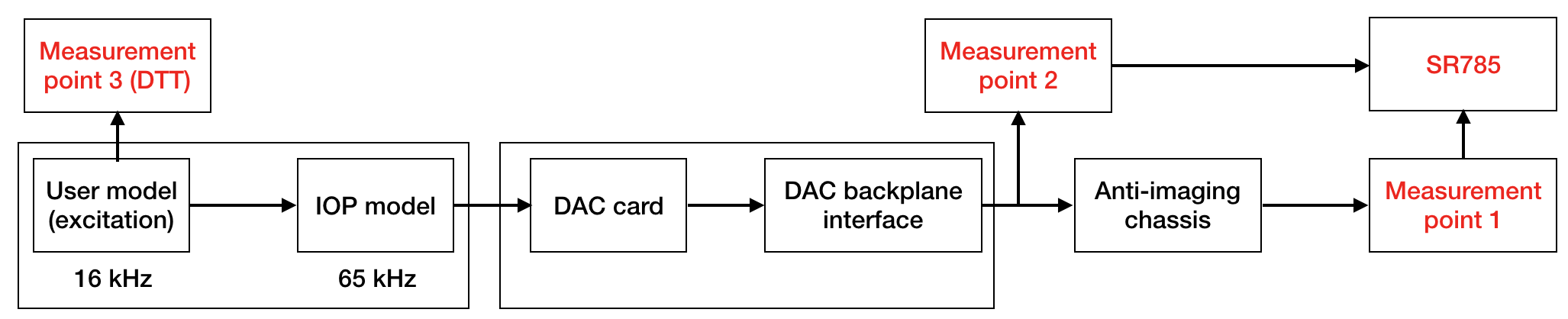
We report on some tests of the 20 and 18 bit DACs performed in the test stand. We drive a signal of varying frequency and amplitude, and check if we see nonlinearities in the spectrum (i.e. lines at multiples of the injected frequency or at other frequencies). The reading is made at the output of the anti-imaging chassis with a break-out board connected to an SR785 (more details about the setup are shown in the first attached image). The following plots have been obtained with the 20-bit DAC, but similar results are observed with the 18 bit DAC.
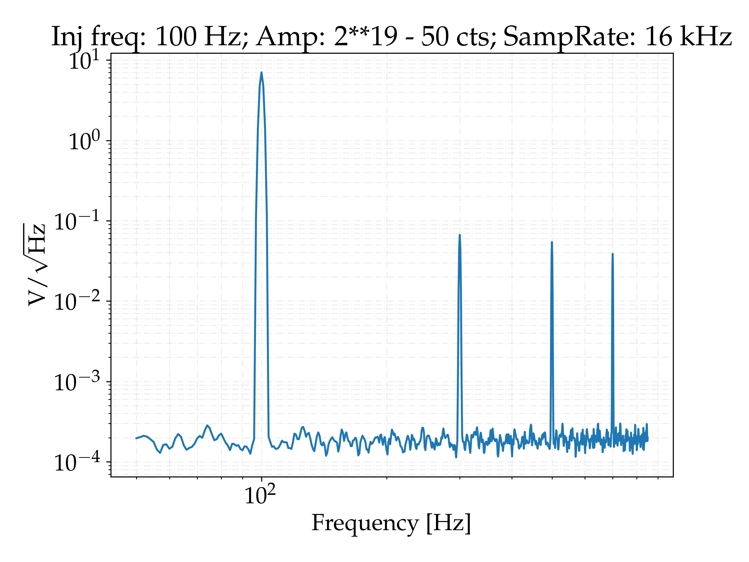
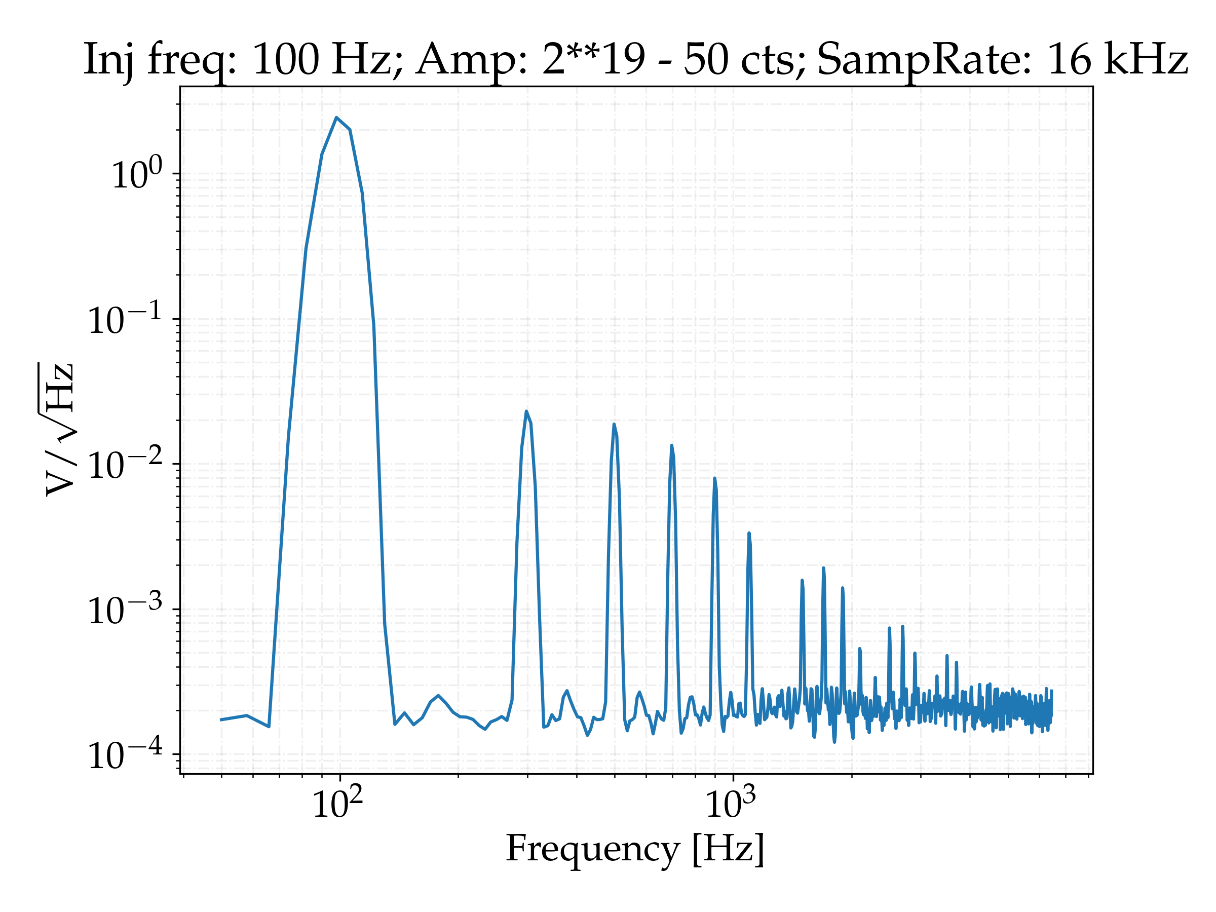
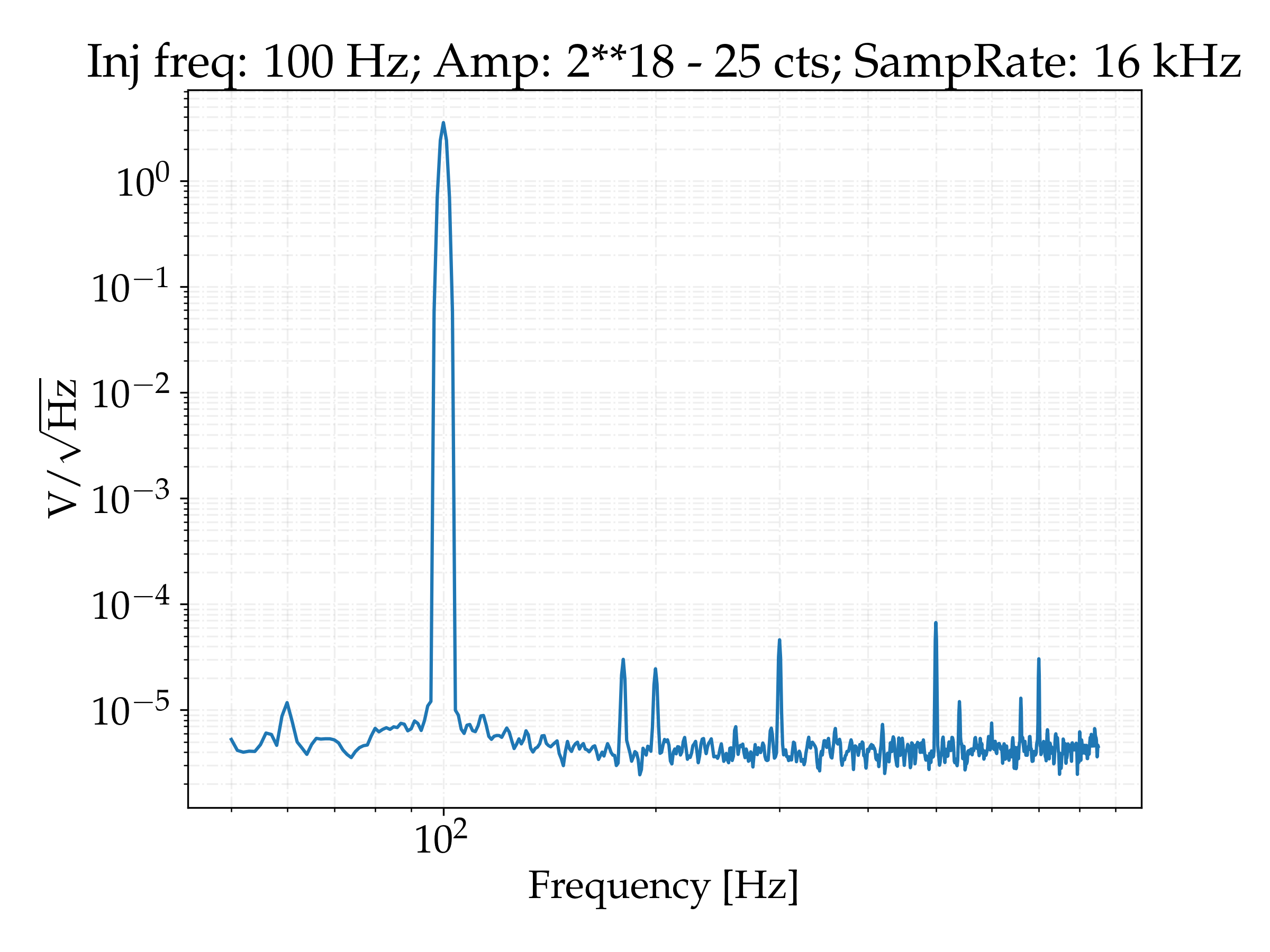
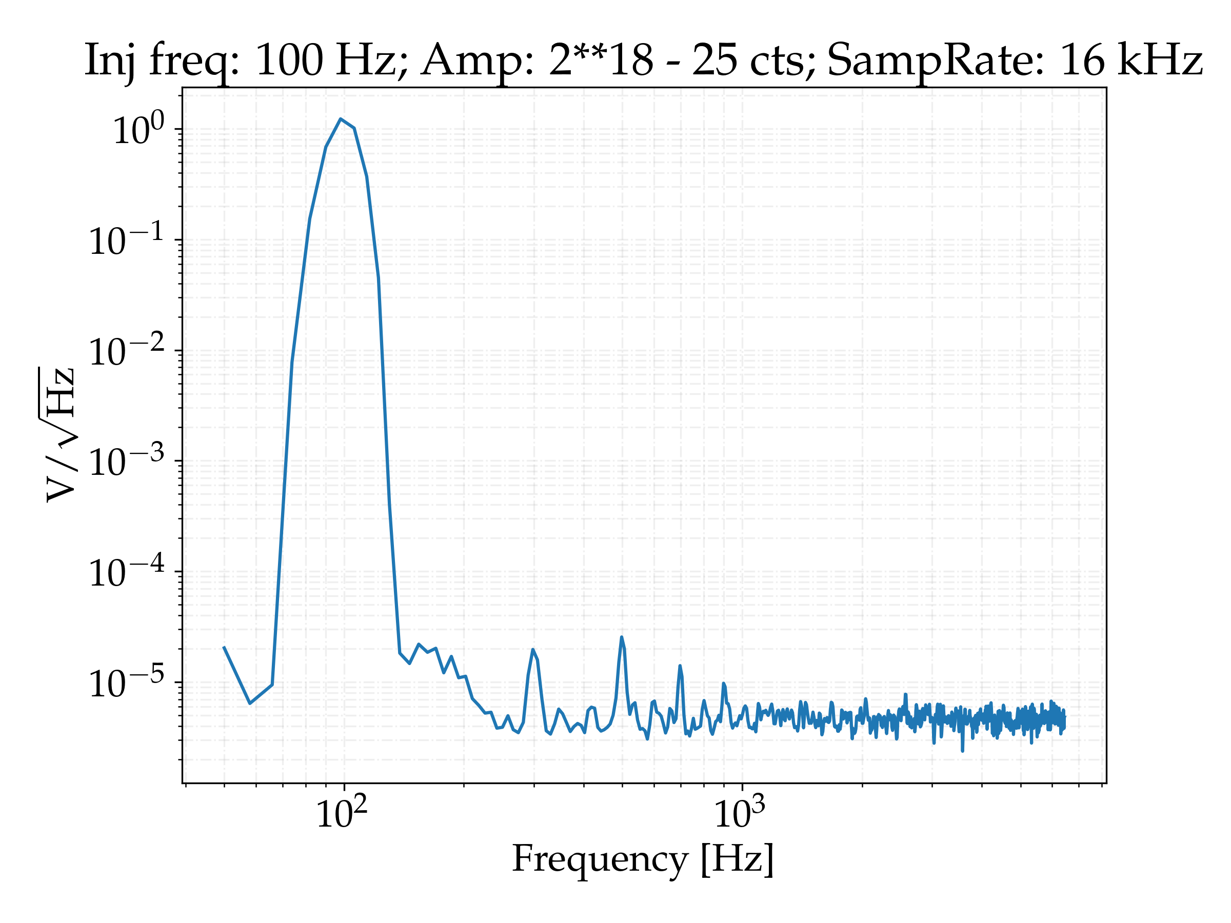
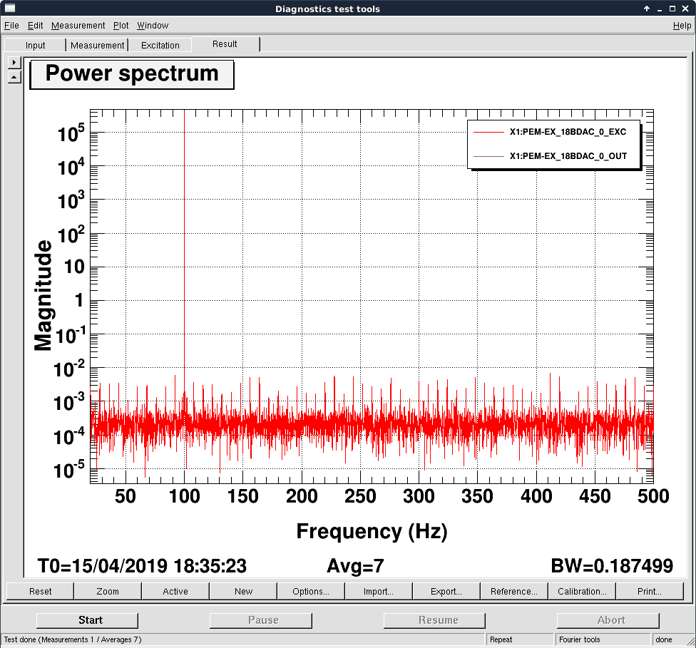
The second figure shows the results obtained by injecting a signal of 100 Hz near the maximum amplitude (~2**19 cts). A comb of lines is produced, with spacing equal to the injected frequency, although only the odd harmonics can be seen. The next figure shows a wider frequency range, where we can see that for frequencies higher than ~4 kHz further harmonics are not visible (the last visible harmonic with an integration time of 10 s is around number 75, but longer integration times make larger harmonics also visible). The next two figures shows the same injected frequency at half number of counts (half amplitude). Many lines can still be seen, at a reduced amplitude than the first figure. In order to not see any of the non-linear lines, the signal amplitude must be lower than ~30000 cts, more than an order of magnitude away from the maximum (with longer integration times this number would be even lower). This comb of lines with spacing equal to the injected frequency is produced at any injected frequency and sampling rate of the user model.
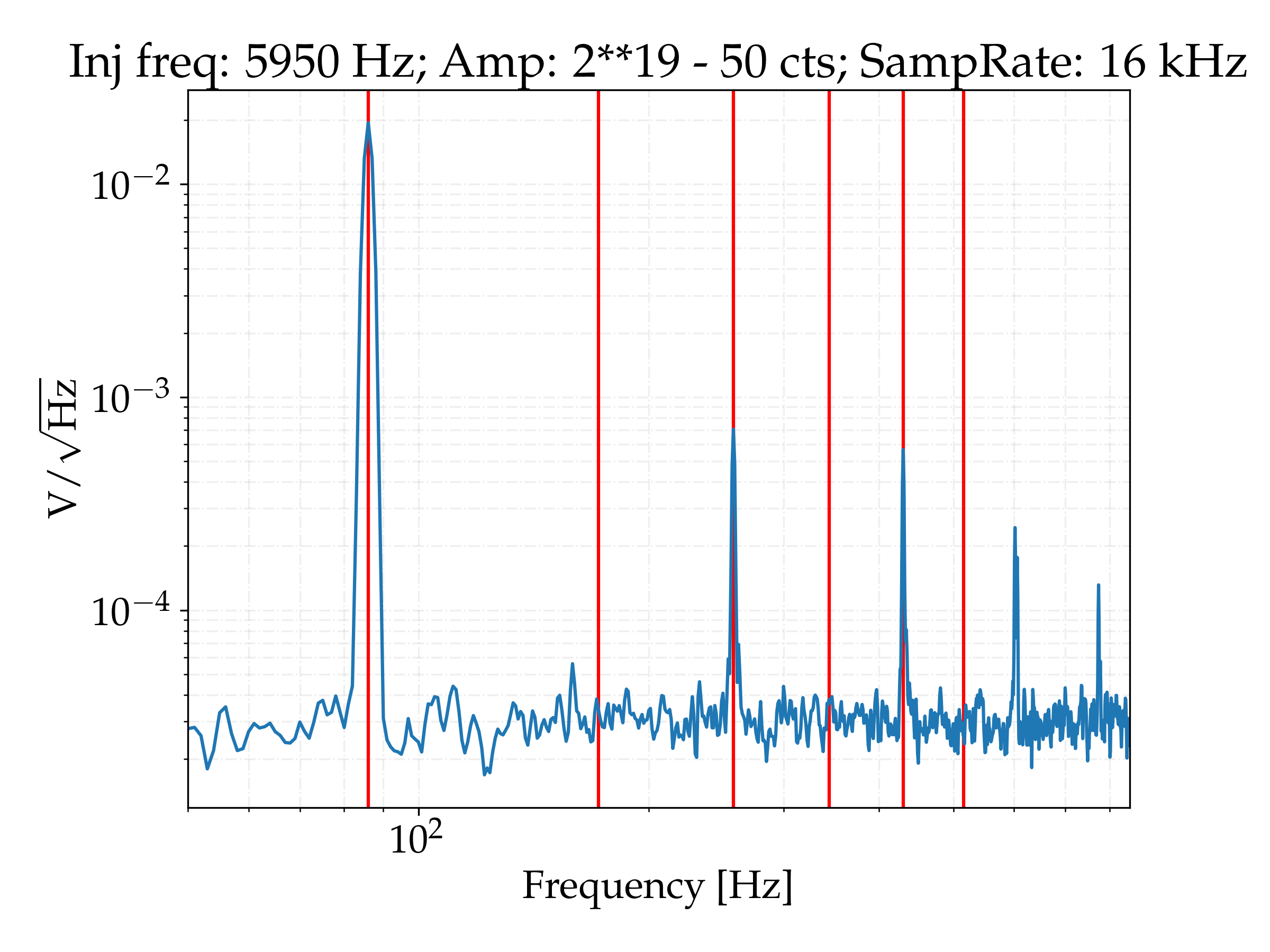
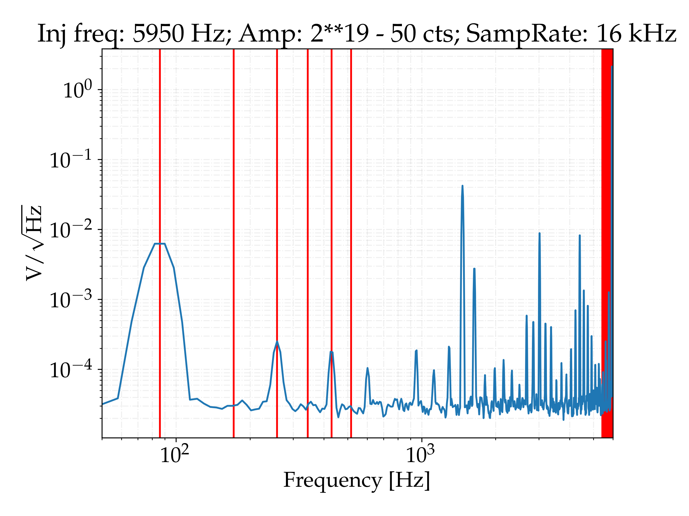
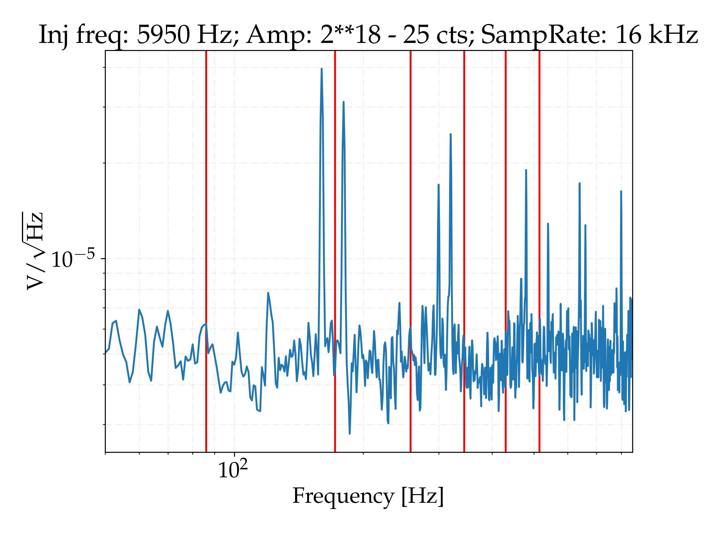
By increasing the frequency of the signal, many lines start to appear in the low frequency range. For example, for a signal of 5950 Hz, lines with a spacing of 86 Hz appear, as shown in the 6th figure (again, only odd harmonics). These lines appear to come from aliasing of the high frequency harmonics of the main comb discussed previously. Harmonics which lie between 2**15 Hz (Nyquist frequency) and 2**16 Hz (sampling rate of IOP model) are ported to the main frequency range by 2**16 - n*freq, where n is the harmonic index. Harmonics between 2**16 and 2**17 are ported by n*freq - 2**16. This pattern is repeated for all the produced harmonics, which get transported to frequencies between 0 and 2**15 Hz. The 5950 Hz frequency has been chosen to replicate the problems discussed in https://alog.ligo-wa.caltech.edu/aLOG/index.php?callRep=37139. Figures 7 and 8 show a wider range of frequencies and the same injection at half amplitude, where the low frequency lines dissappear.
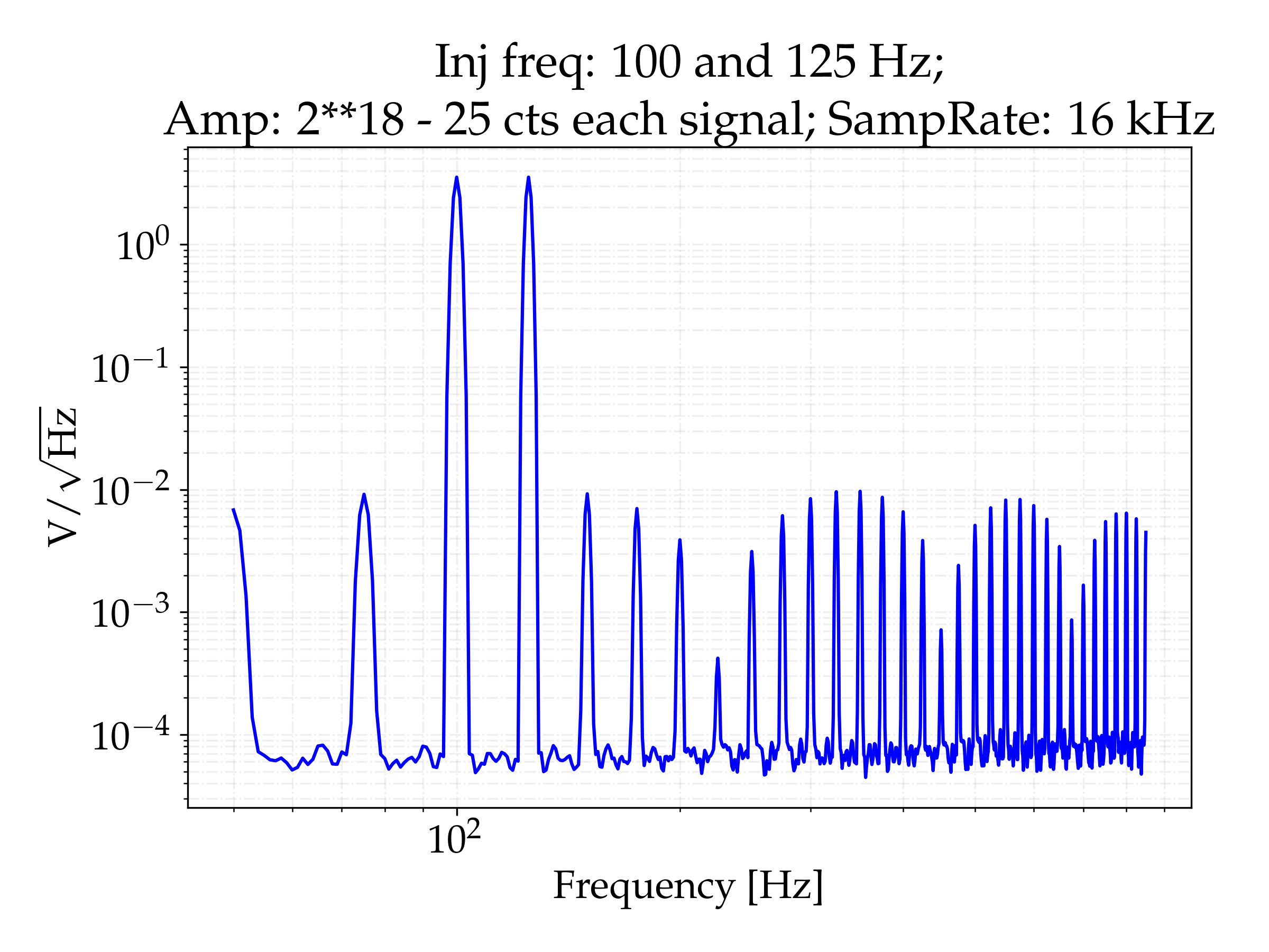
The main comb and the high frequency aliasing explains some of the lines which can be seen, but not all of them. We make further tests by driving two sinusoidal signals of different frequencies at the same time. Plot 9 shows an example of a 100 and 125 Hz signals, where new lines which cannot be seen when only injecting separately 100 or 125 Hz appear. These new lines have a spacing of 25 Hz, suggesting some type of beating between the two injected signals. This beating may explain some of the unexplained lines which appear in the spectrums discussed before. This may also explain some lines seen in DARM at frequencies which seem to be a beating of violin modes and calibration lines, as discussed here: https://alog.ligo-wa.caltech.edu/aLOG/index.php?callRep=48161.
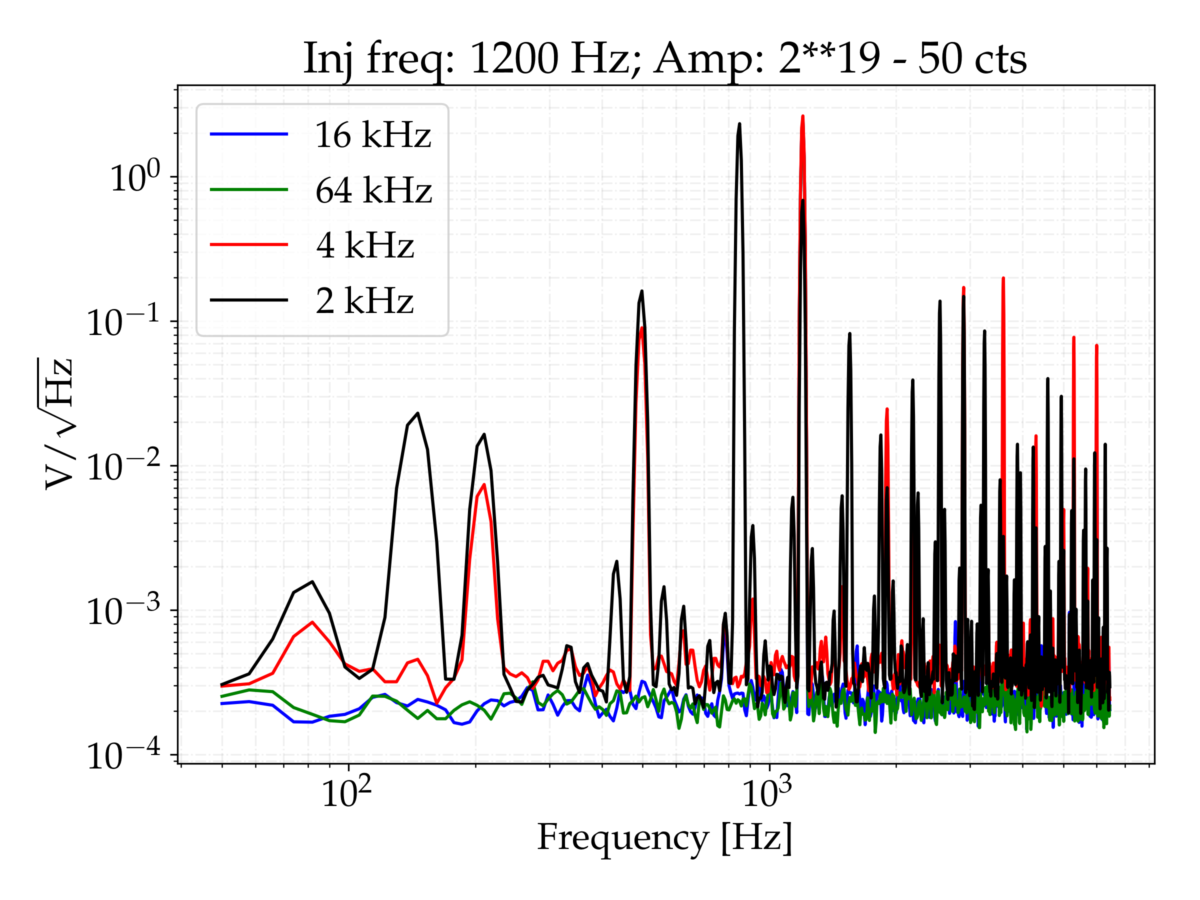
Furthermore, different sampling rates of the user model have been tested. Plot 10 compares the output at different sampling rates. Although the main comb of spacing equal to the injected frequency is there in all the cases, different lines arise for each different sampling rate, with the situation being worse the lowe the sampling rate is.
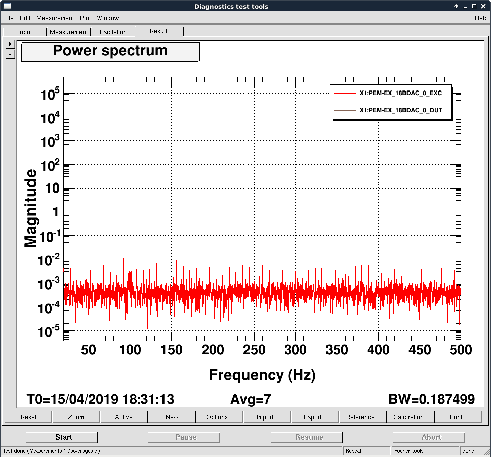
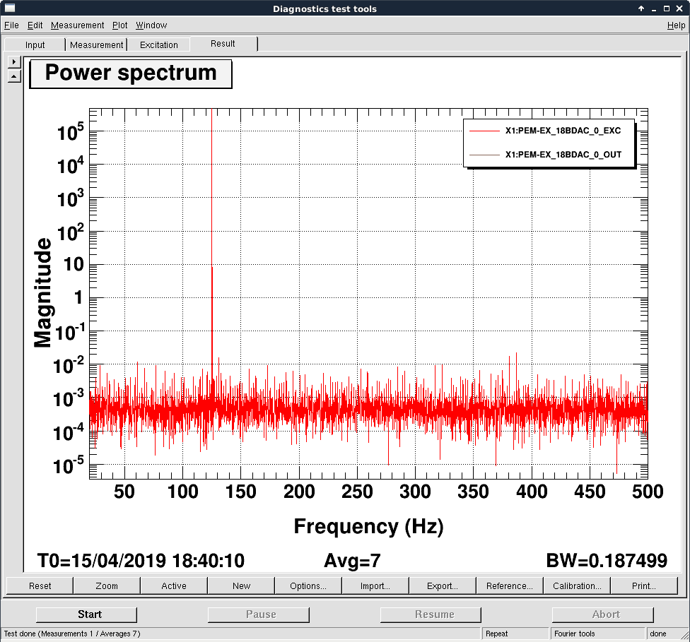
Plots 11-14 show some readings performed at the excitation point with DTT (measurement point 3). Besides the main frequency, a comb of lines can also be seen. The spacing of this comb depends on the frequency of the main injected signal. This is a different feature than the comb which is seen after the DAC and AI, since the main comb of spacing equal to the injected frequency cannot be seen here, neither the beating between multiple injections.
Some readings have also been taken previous to the signal getting into the AI chassis (measurement point 2), and the same lines and nonlinearities have been observed as when measuring from point 1.