[M. Wade, J. Kissel, A. Viets]
Maddie and I have produced new GDS filters for the calibration model update described in LHO aLOGs 54269 and 54473.
I restarted the primary, redundant, and testing calibration pipelines on the DMTs around GPS time 1262990593. Data seems to flowing normally.
The filters are found in revision 9137 of the calibration SVN here:
aligocalibration/trunk/Runs/O3/GDSFilters/H1GDS_1262900044_no_response_corr.npz
They were produced using the run script
aligocalibration/trunk/Runs/O3/H1/Scripts/TDfilters/H1_run_td_filters_1262900044_no_response_corr.sh
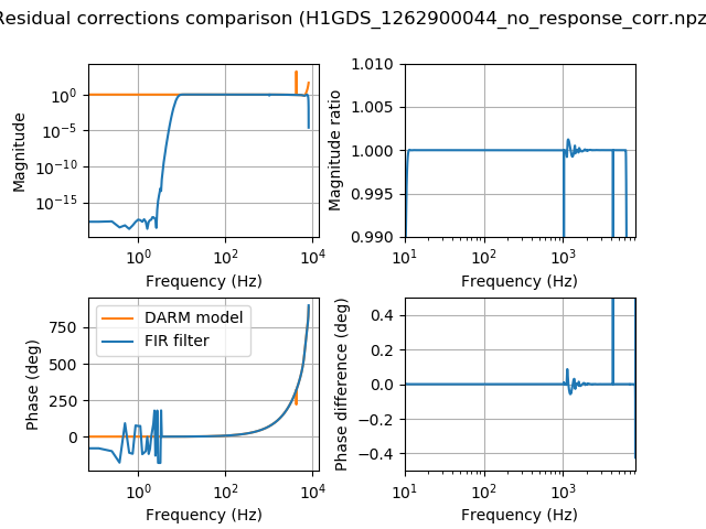
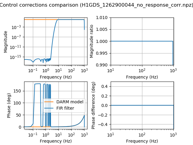
Plots of the frequency response of the filters are attached, comparing them to the frequency-domain model. Note the line at ~4kHz in the resudual corrections filter. This is actually in the control correction model, but it shows up the residual corrections filter plot because we normally apply control corrections above 1kHz in the residual path, since the control path is sampled at only 2kHz. It is surprising to something this large coming from the actuation at such a high frequency. Moreover, modeling this accurately would require a much longer filter sampled at at least 8 kHz, which we do not currently have the computational power to do. Given our skepticism, these filters do not model anything in the actuation above 1 kHz. We have an opportunity tomorrow to update the filters again should we decide that it is a good idea to model this the best we can.
Jeff did a Pcal broadband injection just after the pipelines got running, so once the C00 frames are available, I will add GDS results from that injection. I also plan to test these filters on real data to see how well the model the response function once enough data is available.
The first observation ready segment with the updated calibration model start just now at Jan 14 2020 00:47:59 UTC, or GPS 1262998097.
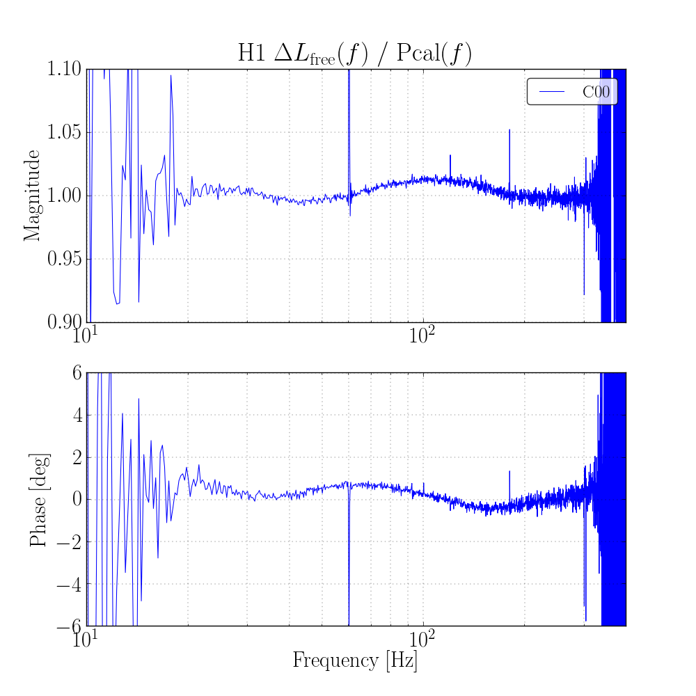
Attached are plots of GDS data during the broadband injection, as well as plots showing how well the filters represent the frequency-domain DARM model. The broadband injection (first plot) looks good, showing deviations no greater than ~2% from 20 Hz - 350 Hz. The last plot shows how well the low-latency (front-end + GDS) calibration pipeline applies the response function R(f). The "spike" seen at 4276.0 Hz is not modeled at all by the filters. The source of this in the model is in all 3 stages of the actuation (only TST and PUM contribute significantly to the response function), and I assume it is a violin mode. This is a very narrow freature in the model, no wider than 0.25 Hz. Models for TST, PUM, and UIM all rise 12 or 13 orders of magnitude at this very narrow feature. We can attempt to model this in the inverse sensing path (which has a high enough sample rate), but it won't be modeled very well if we try, since it is such a narrow feature. Moreover, this would also compromise accuracy in neighboring frequency bins. Most likely, there will still be a loud spectral line in h(t) at 4276 Hz, and the systematic error induced by using the current filters would be that this line appears 3 orders of magnitude lower than it actually is.
Here's a comparison between GDS-CALIB_STRAIN's response to a broadband PCAL Y injection before vs. after this model update. Assuming PCAL is a perfect reference, this should be equivalent to a direct measure of the systematic error in the response function and h(t).

One can see that, while we've cleaned up the UIM feature at 153 Hz, and improved the response ratio below 30 Hz, we seemed to made the systematic error worse between 60 and 150 Hz.

In the first attachment, I show each of the transfer functions on top of each other, to show the former vs. the current level of systematic error.
In the second attachment, I show the ratio of the two transfer functions, to show the *change* in systematic error.

This second attachment should correspond to what Vlad predicted in LHO aLOG 54523. It's close... but not quite right.

Still investigating...

The script used to make this plot can be found here:
    /ligo/svncommon/CalSVN/aligocalibration/trunk/Runs/O3/H1/Scripts/FullIFOSensingTFs/
        plot_GDS_BB_20200115.py
and relies on data processed by Aaron and committed to
    /ligo/svncommon/CalSVN/aligocalibration/trunk/Runs/O3/H1/Results/GDS_BB_plots/
        H1_C00_over_CAL-PCALY_RX_PD_OUT_DQ_1262638969-178.txt
        H1_C00_over_CAL-PCALY_RX_PD_OUT_DQ_1262990871-153.txt

I did some empirical probing into what could be giving this kind of responce between 20 and 300 Hz.
For this I created a new copy of the modelparams_H1_20200103.py file to play with.
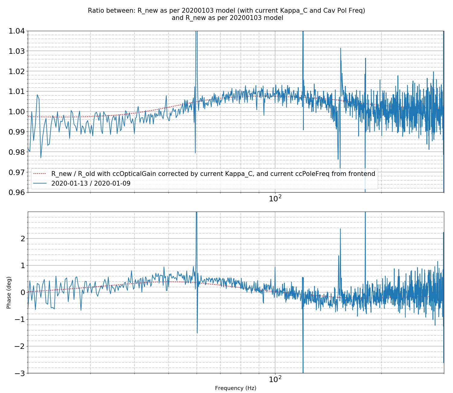
The plot attached here, is where I have taken the ratio of my new version over the currently used version, but I have altered:
- ccOpticalGain is mulitplied by the current Kappa_C written out in the frontend (0.996)
- ccPoleFreq is the current cavity pole frequency in the front end (has minimal effect in this frequency range, but "corrects" for the response change from optical gain at high frequency.
This is plotted against the very data in the above comment, for reference.
It looks like the current systematic error trend can be ?just about? completely explained by this correction! It seems response in this range is *extremely* sensitive to the value of ccOpticalGain in the model.
EDIT: spoke to Jeff - more convincing to reanalyse this w.r.t the Orange line in his figures in the previous comment, and see if it explains the complete error in response.
For reference, here are the values of the TDCFs that were applied to the data in the GDS pipeline during the broadband injections.
During the injection starting at 1262638969:
kappa_tst = 1.0052612
kappa_pum = 1.0198756
kappa_uim = 0.99628365
kappa_C = 0.99136031
f_cc = 411.13184 Hz
During the injection starting at 1262990871:
kappa_tst = 0.99716723
kappa_pum = 1.017796
kappa_uim = 0.99592042
kappa_C = 0.99556768
f_cc = 410.88696 Hz
We needed a better understanding of the impact of this systematic error at ~150 Hz. for the UIM, so I added a copy of ratio plot from LHO aLOG 54565 to the same script,
    ^/trunk/Runs/O3/H1/Scripts/FullIFOSensingTFs/plot_GDS_BB_20200115.py
and zoomed in around the 100-200 Hz frequency region.

Attached are the results.

(1) We're, of course, limited by the frequency resolution and noise of the measurement, BUT,
(2) We see what Vlad has told us all along: there are actually three features: highQ anti-resonance at 151 Hz, highQ anti-resonance at 153 Hz, and then a high Q resonance at 154 Hz (rounding to the nearest Hz). Note that this description is of the *ratio* of (fixed) / (not fixed), so take my description of whether the feature is a "resonance" vs. "anti-resonance" with a grain of salt.
(3) Each highQ feature peaks at around a -2%, -3%, and +3%, BUT -- that includes influence from the "underlying" broad frequency dependent error "sweeping through" this region -- known to be a result of problems with the TST actuator model in this low-latency data.