Evan G., Jeff K.

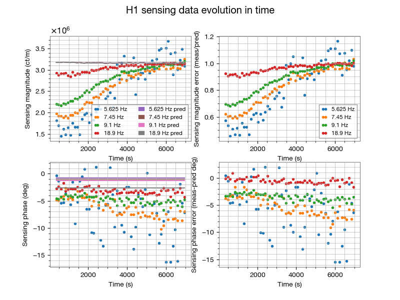
We analyzed the data that Jeff collected at the start of a lock stretch (see LHO aLOG 53951) to understand how the sensing function evolves and impacts the response function as the IFO thermalizes. There were indications that the low frequency part of the sensing function was evolving quite a bit more than we expected. To investigate, Jeff had injected a comb of lines using the PCAL and at the DARM excitation point so that we had a measure of the loop suppression to extract the sensing function.

This data was analyzed offline using gwpy to compute transfer functions at 2 minute intervals in order to plot the changes as a function of time. Typically the sensing function transfer function swept sine measurements are made when the IFO has thermalized. These injections were at fixed frequencies so that we could track the evolution.

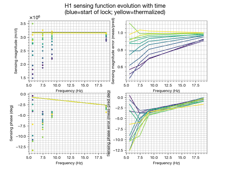
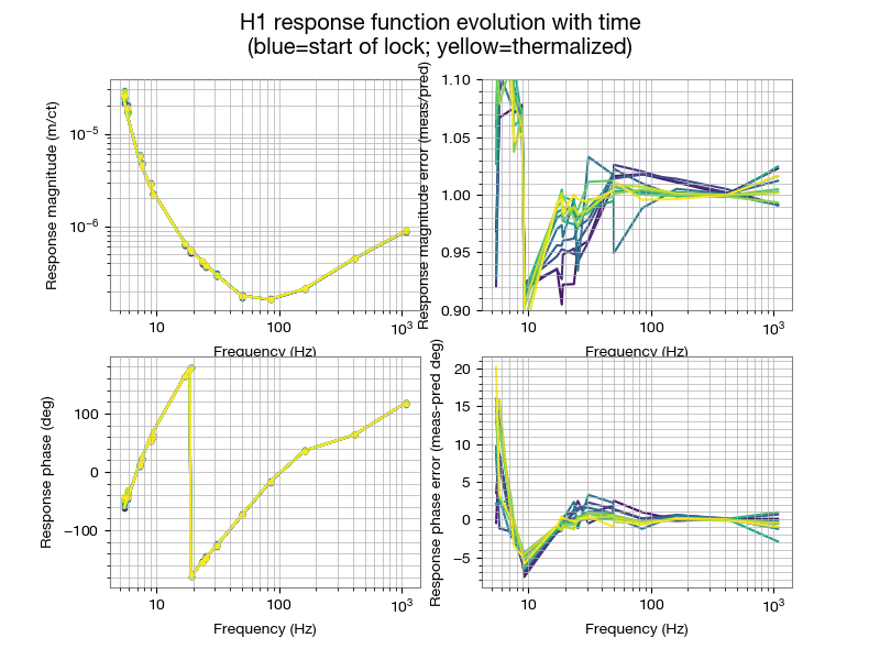
Attached are 8 figures:
1) For the 4 frequencies where the sensing function is measured, we plot the time evolution of the sensing function compared to the pyDARM model predicted using the modelparams_H1_20190909.py file and GDS computed f_cc and kappa_c
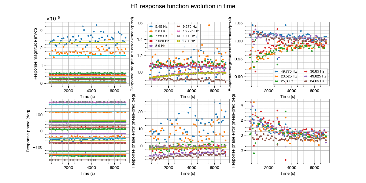
2) For the 18 frequencies where PCAL is injected, we have measured the response function evolution as a function of time compared to the pyDARM model predicted using the modelparams_H1_20190909.py file and GDS computed f_cc and kappa_c
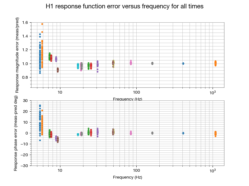
3) For the 18 frequencies where PCAL is injected, we plot the spread of the data points compared to the pyDARM model predicted using the modelparams_H1_20190909.py file and GDS computed f_cc and kappa_c
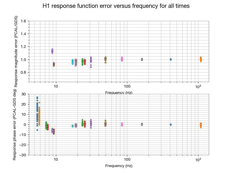
4) For the 18 frequencies where PCAL is injected, we plot the spread of the data points compared to the GDS predicted values (this serves as a check that comparing to pyDARM and the GDS computed values is fine). Note that GDS has a high-pass filter of ~10 Hz
5) Sensing function at intervals of 10 minutes to show the evolution as a function of time (BLUE is the start of the lock, YELLOW is the thermalized IFO state)
6) Response function at intervals of 10 minutes to show the evolution as a function of time (BLUE is the start of the lock, YELLOW is the thermalized IFO state)
7) Sensing function at intervals of 10 minutes to show the evolution as a function of time if one also applies the f_s value as computed by GDS, assuming a Q value of 20 (BLUE is the start of the lock, YELLOW is the thermalized IFO state)
8) Response function at intervals of 10 minutes to show the evolution as a function of time if one also applies the f_s value as computed by GDS, assuming a Q value of 20 (BLUE is the start of the lock, YELLOW is the thermalized IFO state)

The plotting script is in the CAL svn: ^/trunk/Runs/O3/H1/Scripts/FullIFOSensingTFs/process_sensing_20191217_darm_comb.py

The bottom line is in figure 6: at 20 Hz near the beginning of a lock, h(t) is would have a systematic error of ~8% in magnitude and negligible phase. This evolves over the course of ~2 hours, reducing the systematic error close to zero by the end of the 2 hours.

We need to compare this with our current uncertainty estimates and evaluate how to proceed if any interesting triggers are occurring in this 2 hour window at the start of a lock stretch.