Dana, Louis, Jenne

This is a step-by-step guide for how to produce a variety of figures using diaggui (for my future reference and/or other people who are learning this system). I've also included all the relevant information to reproduce the attached figure, where MICH has been calibrated to DARM (both in units of m) so that we can compare how they were affected by an excitation that was injected on June 22nd 2023.

Open a terminal and type diaggui. Make sure nothing is active in the Excitation tab. Then go to the Measurement tab and enter the two channels we want to compare, in this case they are H1:CAL-CS_MICH_DQ and H1:CAL-DELTAL_EXTERNAL_DQ. Make sure both are checked off.

Next set the frequency range to something large, say 0 Hz to 7000 Hz, and change the binwidth (BW) to 0.1 Hz. Also set number of A channels to 2 because we aren't sure yet which channel we want to be our A channel (i.e., which one we want in the denominator of the transfer function; remember if you give it one A channel it will use whichever channel you have in the top, 0th slot, and it counts down from there if you give it more than one A channel).

Then choose a target date, here we used 22/06/2023 at 17:31:26 UTC. Because this is more than a couple months in the past, the data will be stored on tapes so we also need to change the data source. Under the Input tab, switch from Online system to NDS2 and under NDS2 Selection click the dropdown next to Server and choose nds.ligo-wa.caltech.edu. Then go back to the Measurement tab and click start! (If you forget to switch from online to NDS2, the run will stall and never finish but it also won't give you an error message...)

Once it's finished running, go to the Result tab. There will probably be two graphs that are produced, one showing the magnitude in frequency for each channel and one showing the coherence between the two channels. To change to and from log scale and to set axis limits use the Range tab. The position of the legend can also be changed in the Legend tab, and vertical or horizontal cursors can be added using the Cursor tab. To add more panels use the Options tab.

Both power spectra have been whitened, so to undo that we use the Calibration tab. Choose which channel to calibrate, then click New. Reference can be whatever, add proper units (meters in this case), and choose a date that is ideally a bit before the date we've plotted data from. Click Okay and make sure default is checked off. Then for the transfer function information, we used the Pole/Zeros tab for MICH and imported transfer function information for DARM using the Trans. Func. tab. Starting with MICH: Go to sitemap, click on CAL CS, then LSC calib. Click on the transfer function button stemming from the sum of ERR and CTRL; this is the transfer function that did the whitening. To get the poles and zeros, right click somewhere in the background of the window that pops up, then choose Execute and Foton. Then click on the rectangle above the filter (in this case FM2) that was used. DO NOT CLICK ON FM2! This brings up another window which shows the zeros and poles, i.e., zpk, where the first array is the zeros and the second array is the poles. So to undo the whitening, go back to the calibration tab and invert this function, so check off Pole-zero, then type the zeros in the poles box and the poles in the zeros box, each separated by a comma and a space. MICH is measured in um instead of m, so also apply a gain of 1e-6 to convert it to m. Then click Set and Okay. This should have reversed the whitening. For DARM: It is generally the same process, but instead we use the Trans. Func. tab, check off Transfer function, then click Edit and File, Open. Upload a .txt file with the transfer function information, which we grabbed using this command in the terminal:

pydarm export -r 20230621T211522Z --deltal_external_calib_dtt

which returned this:

>>> /var/opt/conda/base/envs/cds/lib/python3.9/site-packages/pandas/core/computation/expressions.py:21: UserWarning: Pandas requires version '2.8.0' or newer of 'numexpr' (version '2.7.3' currently installed).
>>>  from pandas.core.computation.check import NUMEXPR_INSTALLED
>>> INFO | searching for '20230621T211522Z' report...
>>> INFO | found report: 20230621T211522Z
>>> INFO | using model from report: /ligo/groups/cal/H1/reports/20230621T211522Z/pydarm_H1.ini

and created the file /ligo/home/dana.jones/Documents/cal_MICH_to_DARM/deltal_external_calib_dtt.txt.

Now both curves should be calibrated properly. Make sure to save continuously! This should be saved as a .xml file, so later you can reopen it by typing in the terminal diaggui .xml. The file we created is /ligo/home/dana.jones/Documents/cal_MICH_to_DARM/cal_mich_to_darm_11_29_23.xml.

To add a new graph click on the right-pointing arrow next to an empty cell and under the Traces tab use the dropdown next to Graph to tell it what style of graph you want. Check off the Active box and tell it which channel you want, where the convention is B/A. To make the phase plot, go to the Units tab and in the Y dropdown click on Phase (degree).

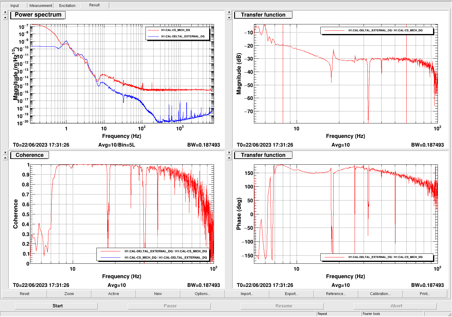
Remember to save one more time when finished. Compare the resulting figure (attached below) to Fig. 3.10 from Jenne's thesis. To review/summarize, the top left panel is showing MICH and DARM during an excitation on June 22nd, the bottom left panel is showing the coherence between MICH and DARM, and the two right panels are showing the magnitude and phase of the transfer function from MICH to DARM.