I'm looking again at the OSEM estimator we want to try on PR3 - see https://dcc.ligo.org/LIGO-G2402303 for description of that idea.
We want to make a yaw estimator, because that should be the easiest one for which we have a hope of seeing some difference (vertical is probably easier, but you can't measure it). One thing which makes this hard is that the cross coupling from L drive to Y readout is large.
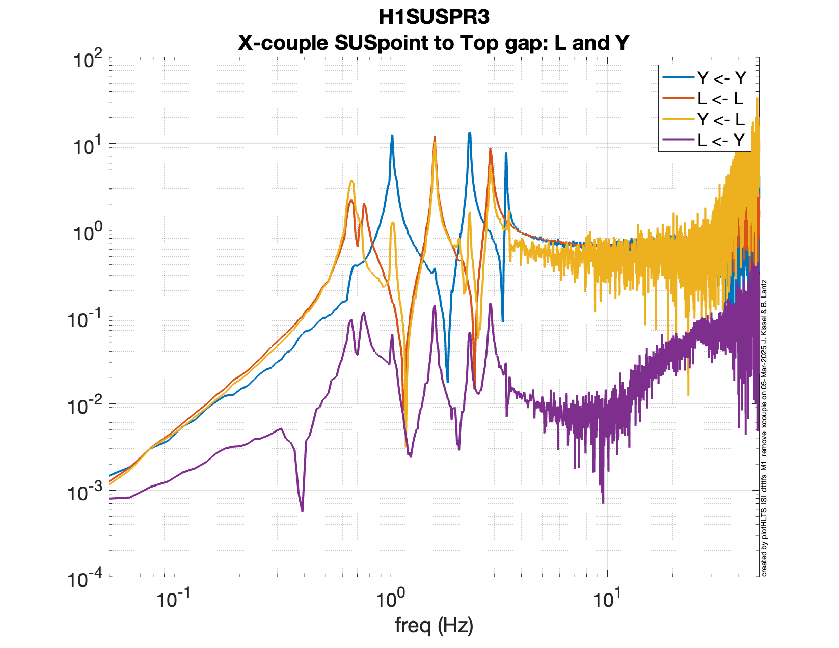
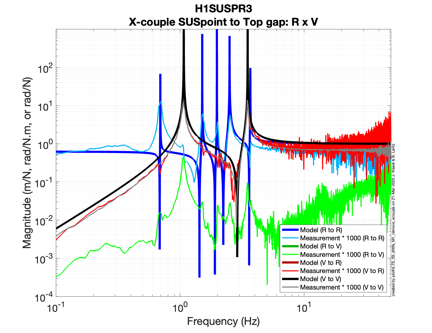
But - a quick comparison (first figure) shows that the L to Y coupling (yellow) does not match the Y to L coupling (purple). If this were a drive from the OSEMs, then this should match. This is actuatually a drive from the ISI, so it is not actually reciprocal - but the ideas are still relevant. For an OSEM drive - we know that mechanical systems are reciprocal, so, to the extent that yellow doesn't match purple, this coupling can not be in the mechanics.
Never-the-less, the similarity of the Length to Length and the Length to Yaw indicates that there is likely a great deal of cross-coupling in the OSEM sensors. We see that the Y response shows a bunch of the L resonances (L to L is the red TF); you drive L, and you see L in the Y signal. This smells of a coupling where the Y sensors see L motion. This is quite plausible if the two L OSEMs on the top mass are not calibrated correctly - because they are very close together, even a small scale-factor error will result in pretty big Y response to L motion.
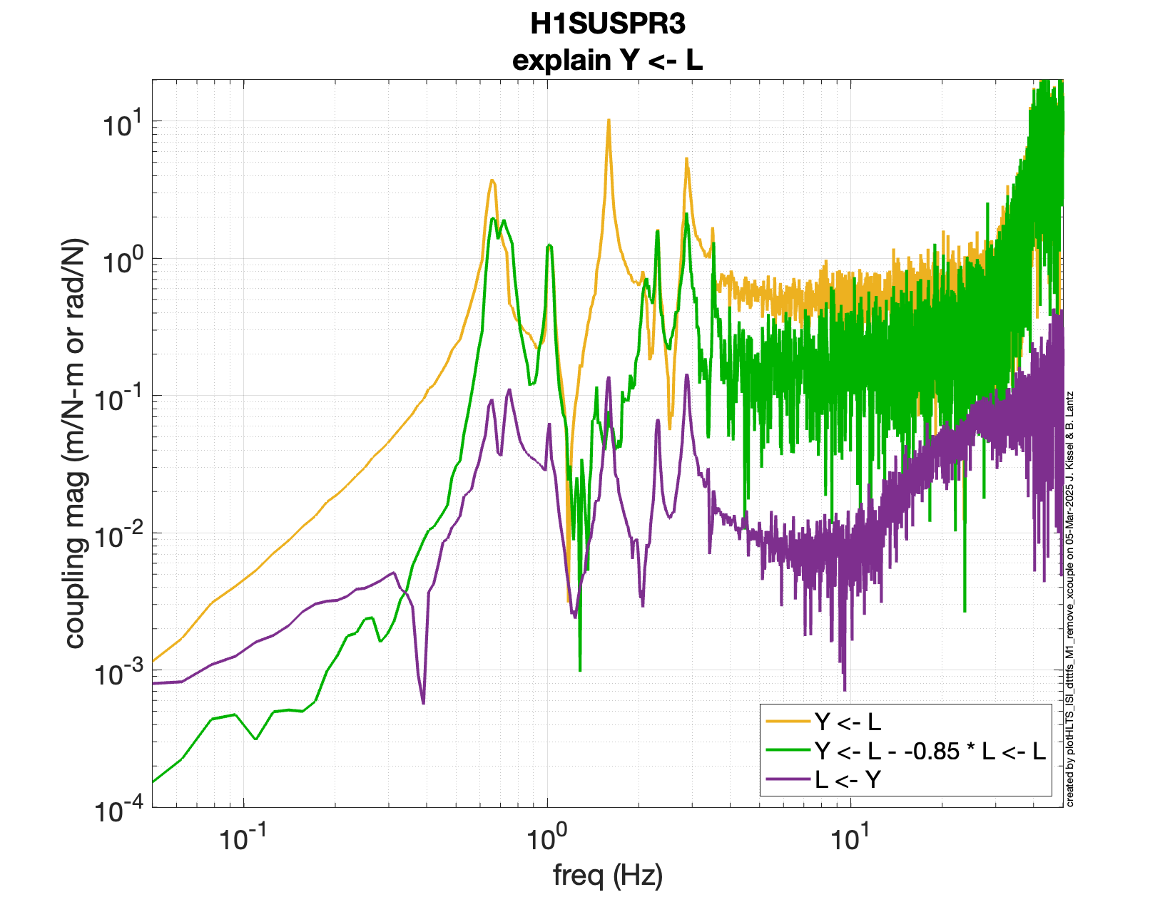
Next - I did a quick fit (figure 2). I took the Y<-L TF (yellow, measured back in LHO alog 80863) and fit the L<-L TF to it (red), and then subtracted the L<-L component. The fit coefficient which gives the smallest response at the 1.59 Hz peak is about -0.85 rad/meter.
In figure 3, you can see the result in green, which is generally much better. The big peak at 1.59 Hz is much smaller, and the peak at 0.64 is reduced. There is more from the peak at 0.75 (this is related to pitch. Why should the Yaw osems see Pitch motion? maybe transverse motion of the little flags? I don't know, and it's going to be a headache).
The improved Y<-L (green) and the original L<-Y (purple) still don't match, even though they are much closer than the original yellow/purple pair. Hence there is more which could be gained by someone with more cleverness and time than I have right now.
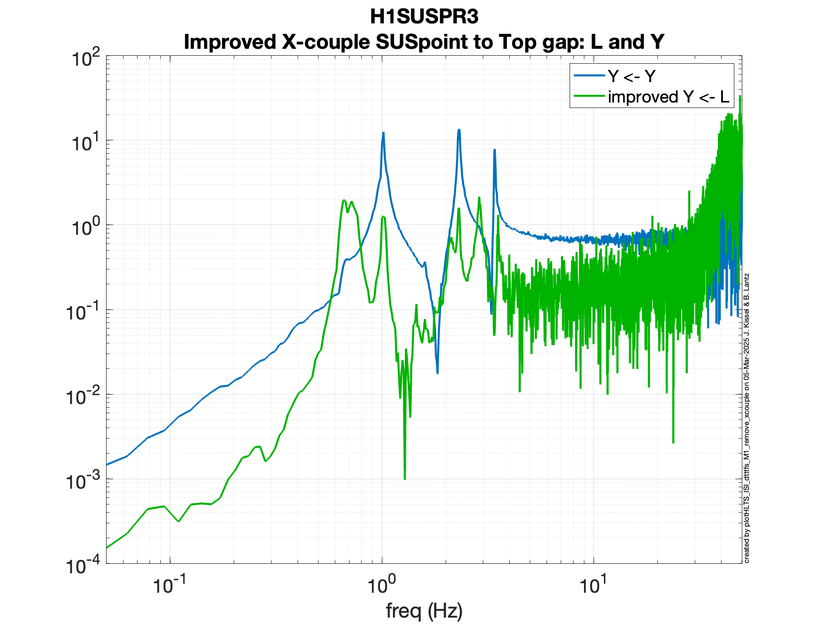
figure 4 - I've plotted just the Y<-Y and Y<-L improved.
Note - The units are wrong - the drive units are all meters or radians not forces and torques, and we know, because of the d-offset in the mounting of the top wires from the suspoint to the top mass, that a L drive of the ISI has first order L and P forces and torques on the top mass. I still need to calculate how much pitch motion we expect to see in the yaw reponse for the mode at 0.75 Hz.
In the meantime - this argues that the yaw motion of PR3 could be reduced quite a bit with a simple update to the SUS large triple model, I suggest a matrix similar to the CPS align in the ISI. I happen to have the PR3 model open right now because I'm trying to add the OSEM estimator parts to it. Look for an ECR in a day or two...
This is run from the code {SUS_SVN}/HLTS/Common/MatlabTools/plotHLTS_ISI_dtttfs_M1_remove_xcouple'
-Brian
ah HA! There is already a SENSALIGN matrix in the model for the M1 OSEMs - this is a great place to implement corrections calculated in the Euler basis. No model changes are needed, thanks Jeff!
If this is a gain error in 1 of the L osems, how big is it? - about 15%.
Move the top mass, let osem #1 measure a distance m1, and osem #2 measure m2.
Give osem #2 a gain error, so it's response is really (1+e) of the true distance.
Translate the top mass by d1 with no rotation, and the two signals will be m1= d1 and m2=d1*(1+e)
L is (m1 + m2)/2 = d1/2 + d1*(1+e)/2 = d1*(1+e/2)
The angle will be (m1 - m2)/s where s is the separation between the osems.
I think that s=0.16 meters for top mass of HLTS (from make_sus_hlts_projections.m in the SUS SVN)
Angle measured is (d1 - d1(1+e))/s = -d1 * e /s
The angle/length for a length drive is
-(d1 * e /s)/ ( d1*(1+e/2)) = 1/s * (-e/(1+e/2)) = -0.85 in this measurement
if e is small, then e is approx = 0.85 * s = 0.85 rad/m * 0.16 m = 0.14
so a 14% gain difference between the rt and lf osems will give you about a 0.85 rad/ meter cross coupling. (actually closer to 15% -
0.15/ (1 + 0.075) = 0.1395, but the approx is pretty good.
15% seem like a lot to me, but that's what I'm seeing.
I'm adding another plot from the set to show vertical-roll coupling.
fig 1 - Here, you see that the vertical to roll cross-couping is large. This is consistent with a miscalibrated vertical sensor causing common-mode vertical motion to appear as roll. Spoiler-alert - Edgard just predicted this to be true, and he thinks that sensor T1 is off by about 15%. He also thinks the right sensor is 15% smaller than the left.
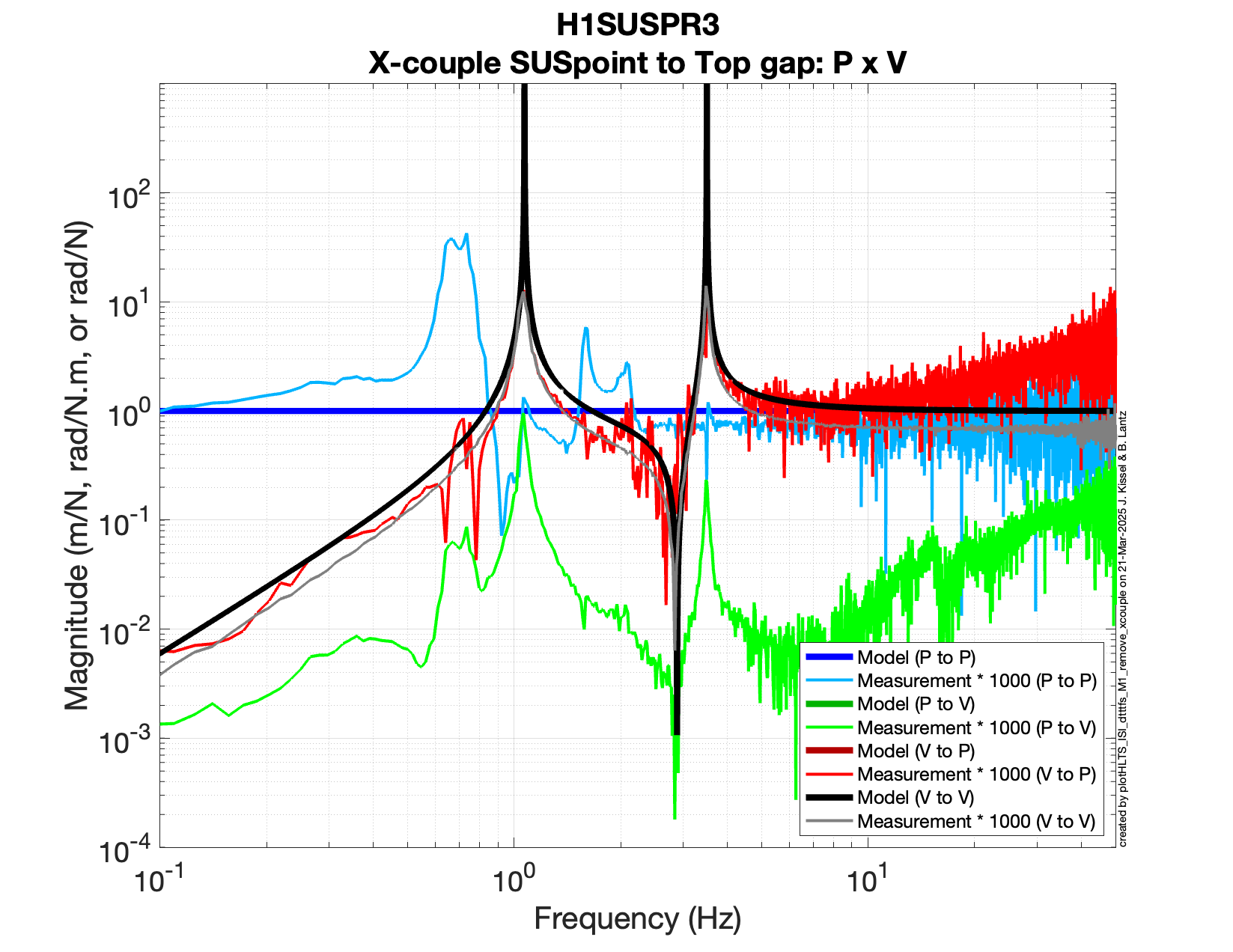
-update-
fig 2- I've also added the Vertical-Pitch plot. Here again we see significant response of the vertical motion in the Pitch DOF. We can compare this with what Edgard finds. This will be a smaller difference becasue the the pitch sensors (T2 and T3, I think) are very close together (9 cm total separation, see below).
Here are the spacings as documented i the SUS_SVN/HLTS/Common/MatlabTools/make_sushlts_projections.m
I was looking at the M1 ---> M1 transfer functions last week to see if I could do some OSEM gain calibration.
The details of the proposed sensor rejiggling is a bit involved, but the basic idea is that the part of the M1-to-M1 transfer function coming from the mechanical plant should be reciprocal (up to the impedances of the ISI). I tried to symmetrize the measured plant by changing the gains of the OSEMs, then later by including the possibility that the OSEMs might be seeing off-axis motion.
Three figures and three findings below:
0) Finding 1: The reciprocity only allows us to find the relative calibrations of the OSEMs, so all of the results below are scaled to the units where the scale of the T1 OSEM is 1. If we want absolute calibrations, we will have to use an independent measurement, like the ISI-->M1 transfer functions. This will be important when we analyze the results below.
1) Figure 1: shows the full 6x6 M1-->M1 transfer function matrix between all of the DOFs in the Euler basis of PR3. The rows represent the output DOF and the columns represent thr input DOF. The dashed lines represent the transpose of the transfer function in question for easier comparison. The transfer matrix is not reciprocal.
2) Finding 2: The diagonal correction (relative to T1) is given by:
0 0.89 0 0 0 0 T2
0 0 0.84 0 0 0 T3
0 0 0 0.86 0 0 LF
0 0 0 0 1 0 RT
0 0 0 0 0 0.84 SD
0.085 0.807 0.042 0.005 0.006 0.006 T2
0.096 0.077 0.723 0.013 0.002 0.03 T3
-0.036 0.025 -0.02 0.696 0.012 0.006 LF
-0.004 -0.018 0.045 0.016 0.809 -0.004 RT
-0.035 0.026 0.02 0.004 -0.008 0.815 SD
I will post more analysis in the Euler basis later.

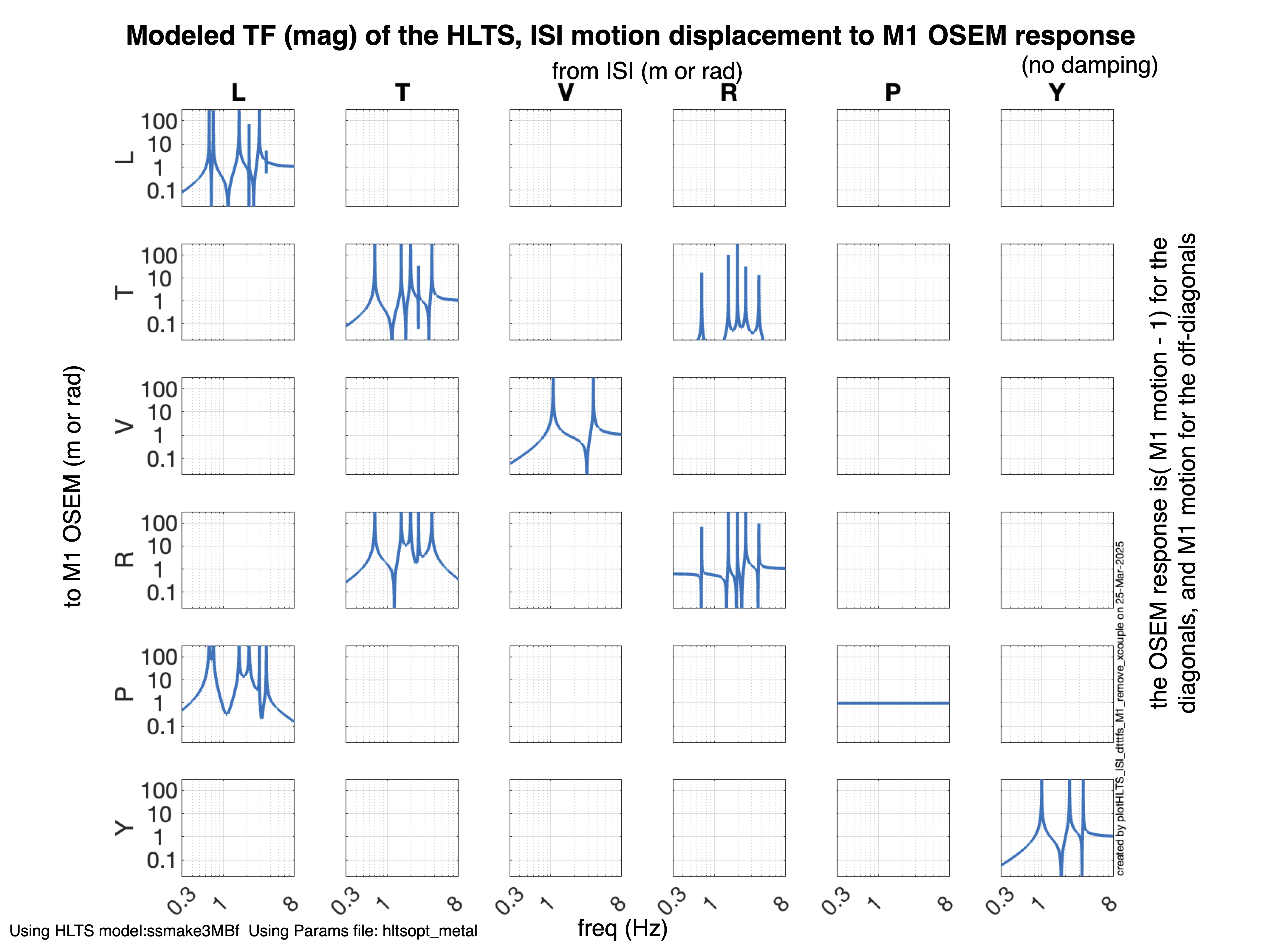
Here's a view of the Plant model for the HLTS - damping off, motion of M1. These are for reference as we look at which cross-coupling should exist. (spoiler - not many)
First plot is the TF from the ISI to the M1 osems.
L is coupled to P, T & R are coupled, but that's all the coupling we have in the HLTS model for ISI -> M1.
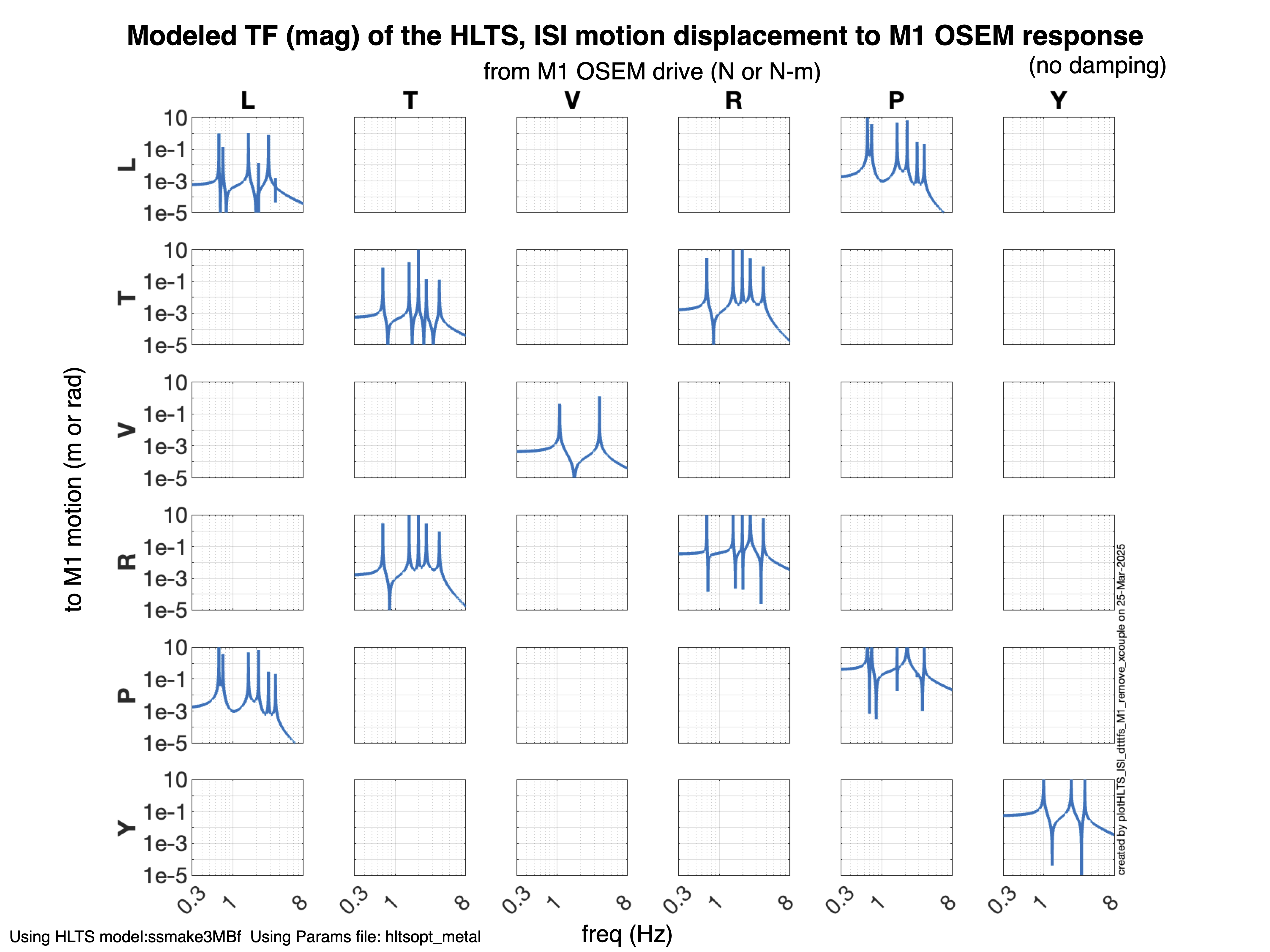
Second plot is the TF from the M1 drives to the M1 osems.
L & P are coupled, T & R are coupled, but that's all the coupling we have in the HLTS model for M1 -> M1.
These plots are Magnitude only, and I've fixed the axes.
For the OSEM to OSEM TFs, the level of the TFs in the blank panels is very small - likely numerical issues. The peaks are at the 1e-12 to 1e-14 level.
@Brian, Edgard -- I wonder if some of this ~10-20% mismatch in OSEM calibration is that we approximate the D0901284-v4 sat amp whitening stage with a compensating filter of z:p = (10:0.4) Hz?
(I got on this idea thru modeling the *improvement* to the whitening stage that is already in play at LLO and will be incoming into LHO this summer; E2400330)

If you math out the frequency response from the circuit diagram and component values, the response is defined by
    %  Vo                         R180
    % ---- = (-1) * --------------------------------
    %  Vi           Z_{in}^{upper} || Z_{in}^{lower}
    %
    %               R181   (1 + s * (R180 + R182) * C_total)
    %      = (-1) * ---- * --------------------------------
    %               R182      (1 + s * (R180) * C_total)
So for the D0901284-v4 values of
    R180 = 750;
    R182 = 20e3;
    C150 = 10e-6;
    C151 = 10e-6;

    R181 = 20e3;

that creates a frequency response of
    f.zero = 1/(2*pi*(R180+R182)*C_total) = 0.3835 [Hz];
    f.pole = 1/(2*pi*R180*C_total) = 10.6103 [Hz];


I attach a plot that shows the ratio of the this "circuit component value ideal" response to approximate response, and the response ratio hits 7.5% by 10 Hz and ~11% by 100 Hz.

This is, of course for one OSEM channel's signal chain.

I haven't modeled how this systematic error in compensation would stack up with linear combinations of slight variants of this response given component value precision/accuracy, but ...

... I also am quite confident that no one really wants to go through an measure and fit the zero and pole of every OSEM channel's sat amp frequency response, so maybe you're doing the right thing by "just" measuring it with this technique and compensating for it in the SENSALIGN matrix. Or at least measure one sat amp box's worth, and see how consistent the four channels are and whether they're closer to 0.4:10 Hz or 0.3835:10.6103 Hz.

Anyways -- I thought it might be useful to be aware of the many steps along the way that we've been lazy about the details in calibrating the OSEMs, and this would be one way to "fix it in hardware."