Today, we measured the calibration at three different ESD biases. First, we measured at the current bias of 269 V, and then our O4 standard bias of 136 V. Then, I stepped up to a higher bias of 409 V.
| ESDAMON value | Bias Offset | L3 Drivealign gain | Calibration report | Notes |
| 269 V | 6.0542453 | 88.28457 |
alog: 86337 report: 20250813T153848Z |
only 1 hour thermalized at measurement time current operating bias |
| 136 V | 3.25 | 198.6643 |
alog: 86339 report: 20250813T162026Z |
nominal O4 bias, calibration model fit at this bias |
| 409 V | 8.89 | 57.587 |
alog: 86341 report: 20250813T174921Z |
ESD saturation warnings while at this bias Took 5 minutes of quiet time, cal lines on, at this new bias start: 18:12:54 UTC end: 18:18:00 UTC |
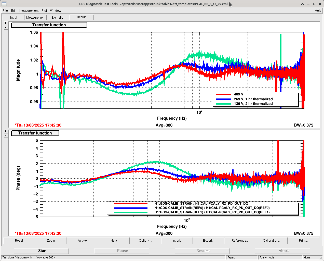
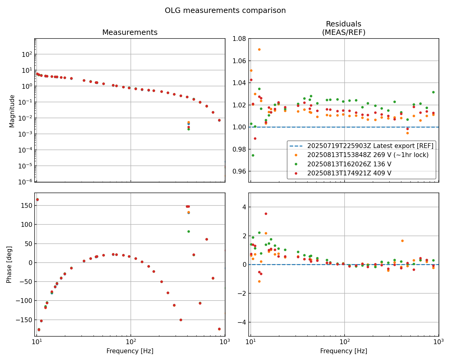
The attached plot compares the three broadband measurements at each ESD bias. It seems like the overall systematic error decreases as we increase the ESD bias.
To step up the ESD bias, I used guardian code that Sheila attached to this alog. Another relevant alog comparing simulines results at different biases is here.
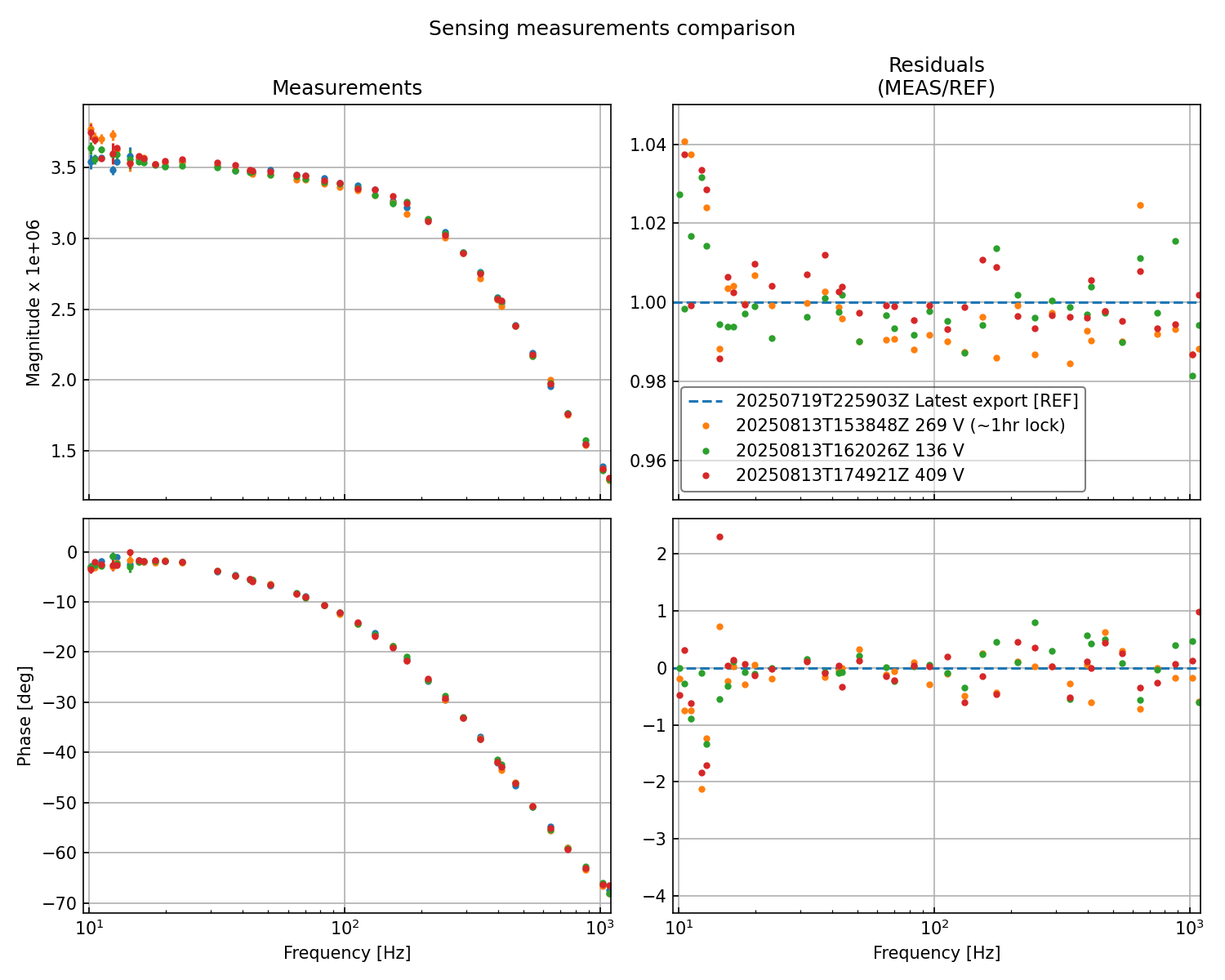
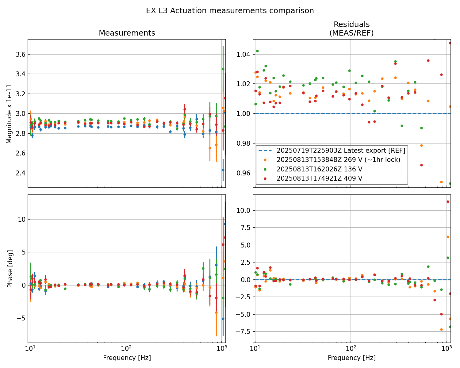
Attaching figures comparing the sensing function, the actuation function, and the open loop gain (olg). All the figures are formatted in the same way, where the left side shows the bode plot from each report and the right shows the bode plot from of each measurement ratio to a reference. I used the latest exported calibration measurement "20250719T225835Z" as a reference. From 10 Hz to 1 kHz the sensing and the actuation function residuals are within 5%. The OLG is within 10% with one outlier at 410 Hz.
We are trying to understand how the systematic error is changing at each bias voltage, even though we think we are correcting the drivealign gain to account for the actuation change.
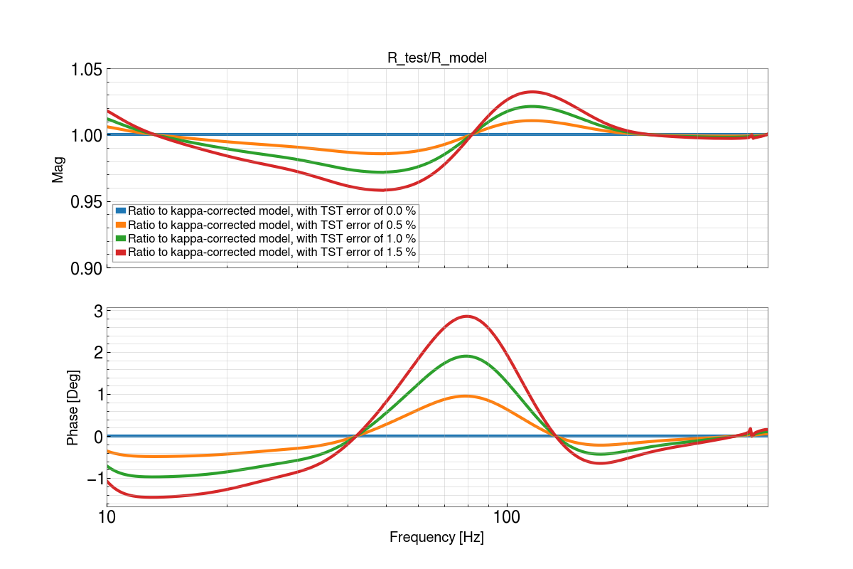
Francisco and I made some plots of how the modeled error changes. First, we pulled the model from the 20250719T225835Z report, since that is our current calibration model. Then, we pulled the kappas at the time of the lowest bias voltage measurement, since that is the bias voltage that our model is based on. We applied the kappas from that measurement time, and then calculated a new response function assuming an additional TST actuation change, ranging from no change (0%) to 1.5% change. Then, we compared each of these response functions to the kappa-corrected model.
To be clear, we are calculating the new response function as:
R = 1/C_model + (error_factor*TST_model + PUM_model + UIM_model) * D_model
The "model" in this case also has the kappa-corrected values applied, which are:
{'c': 0.98335475,
'f_c': 447.65558,
'uim': 1.0052187,
'pum': 1.0012773,
'tst': 1.0183398}
Looking at our results side-by-side with the broadband pcal measurement, we see some similarites. However, it's not exactly the same, since the frequency dependence appears slightly different in the measurement than the model.
There are some other comparisons to be made, but we can start with these. The script I used to make this plot is saved in /ligo/groups/cal/H1/ifo/scripts/compare_models_tst_err.py