Setting Lens Position for SPI In-vac SuK Fiber Collimator Beam Profile: No Systematic Error; Waist Position is just *extremely* Sensitive to Lens position

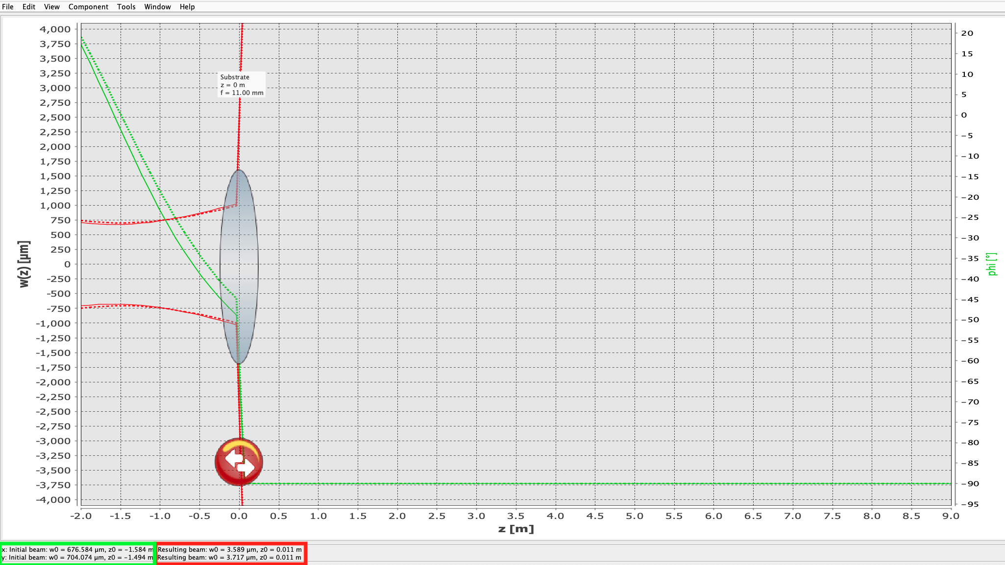
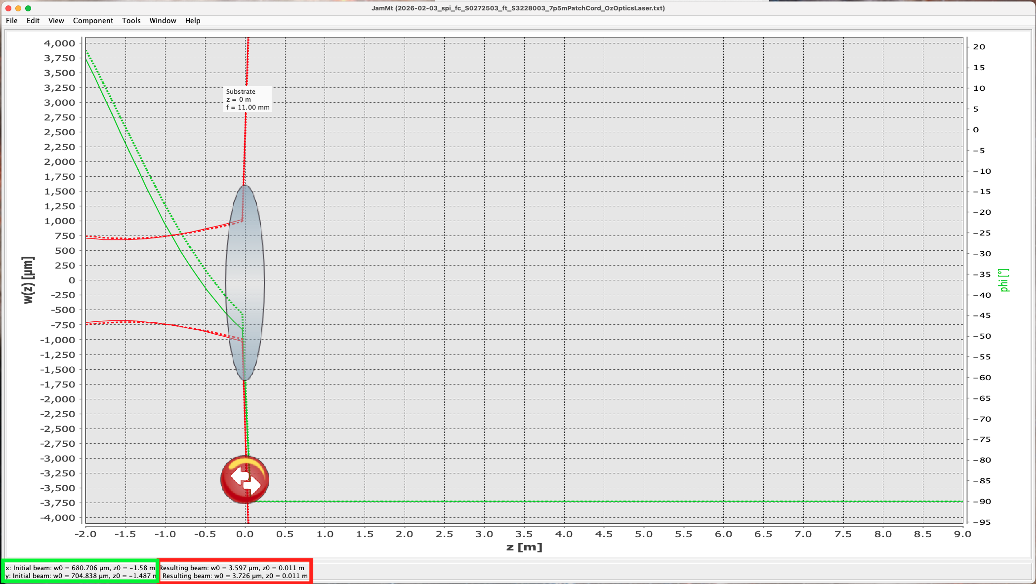
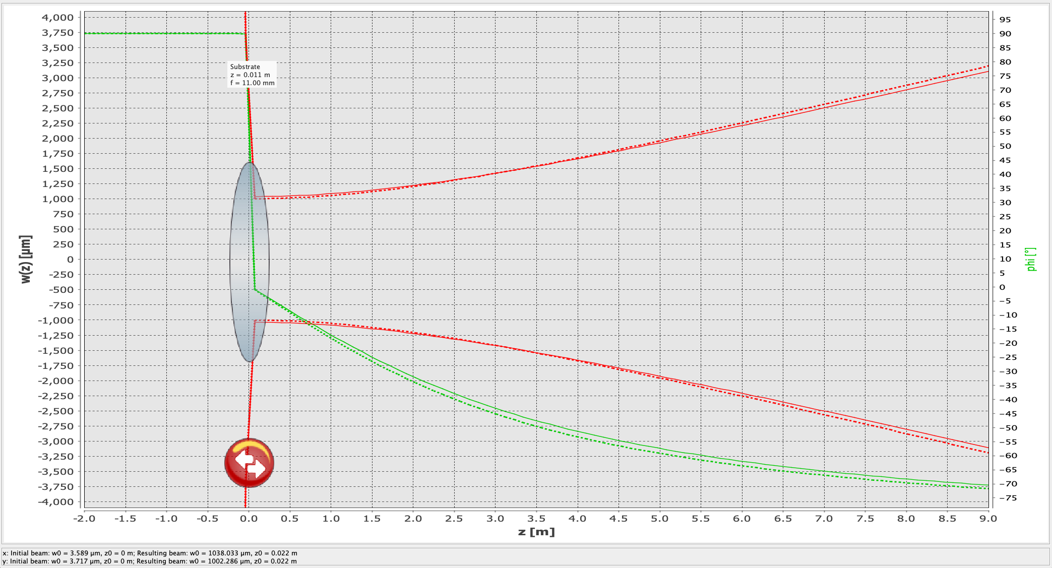
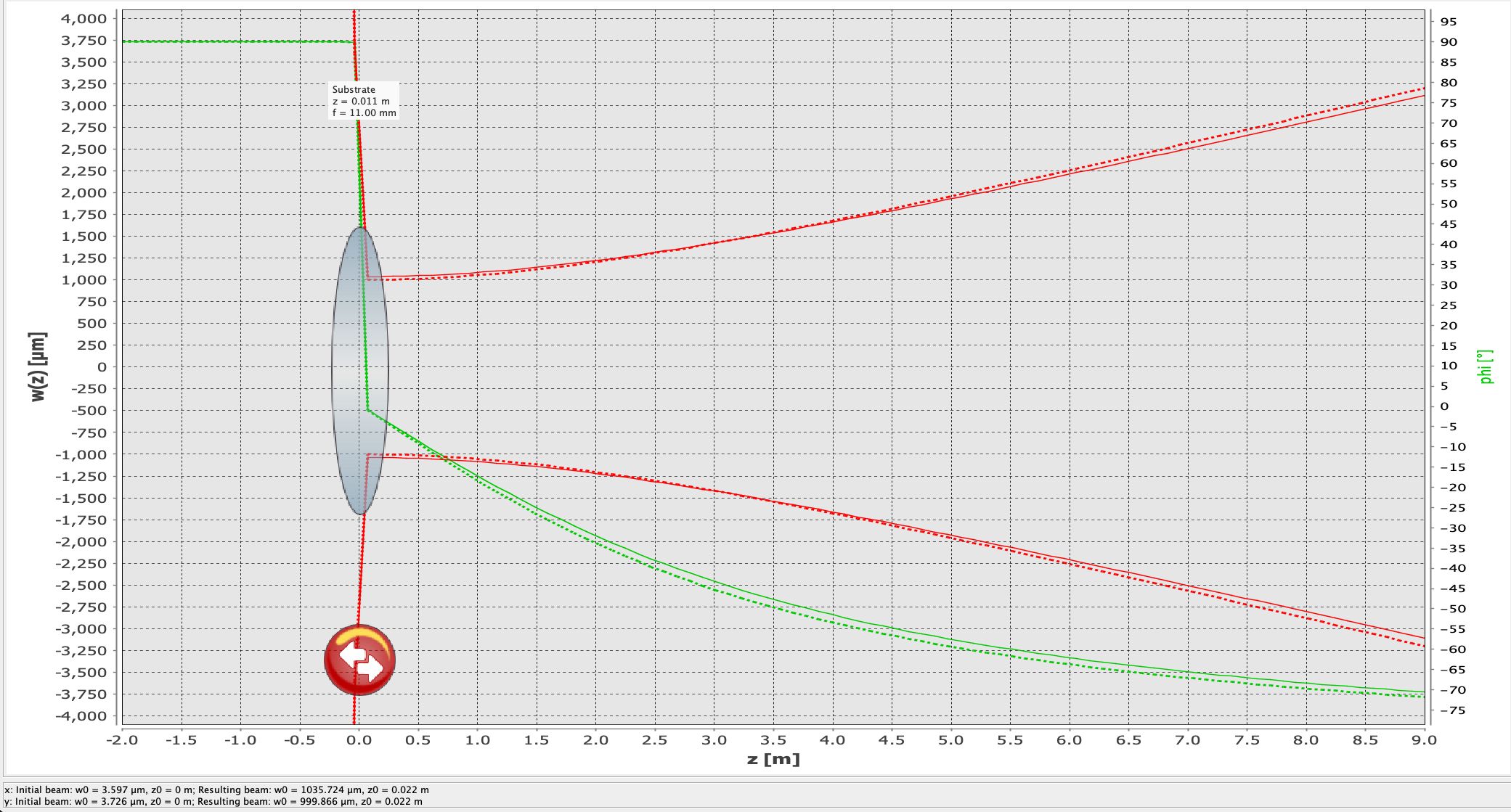
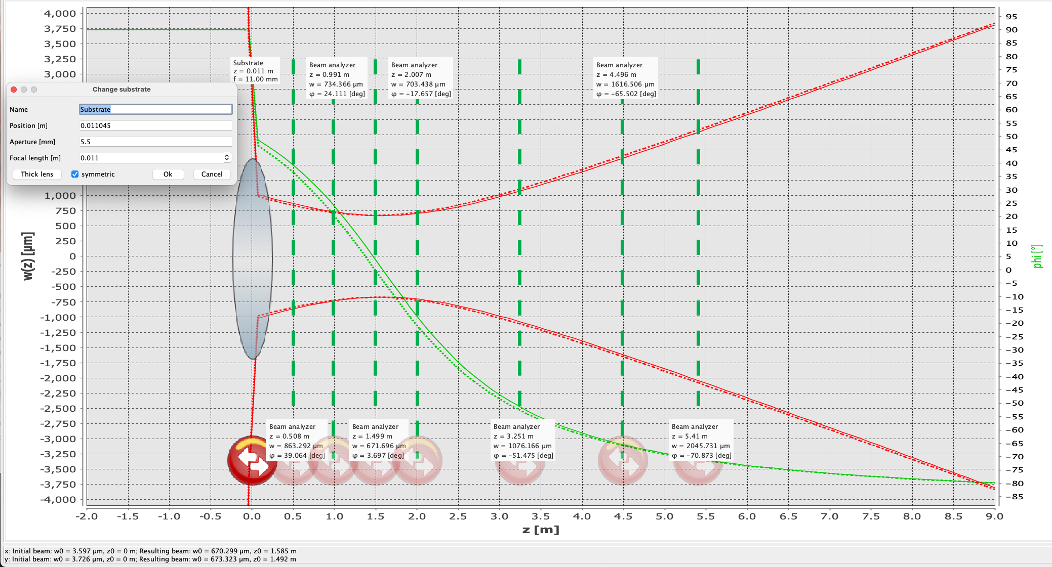
J. Kissel, S. Koehlenbeck

Executive Summary: after some more modeling of the beam profiles from LHO:89047, we identify that there's nothing fundamentally wrong in the analysis -- it's just that the out-going waist position of the beam exiting the SPI fiber collimators is just *extremely* sensitive to lens position -- to the tune of z_lens = 11 [mm] +/- 50 [um] can swing the waist position z0 = +/- 1.5 [m], and that makes it extremely challenging to set the waist at z0 = 0.0 [m] with out a better measurement setup/method for adjusting the position.

The full story:

Trying to better understand the results from LHO:89047, in this aLOG I:

(0) Verified Beam Profile Fit with JAMMT instead of A La Mode: Imported the beam profile data from each laser into JaMMT, with the z-axis inverted (i.e. z = [-5.41, -4.496, ... , -0.508] [m]), and confirmed that JaMMT agrees with a la mode in terms of waist radius, w0, and waist position, z0 -- except now with the beam "incoming" into the collimator/lens/fiber.
The fit predicts a waist w0 at position z0 of 
                               JaMMT                           A La Mode (Matlab)
                           w0y'     w0x'                        w0x     w0y            (assume w0x = w0y', w0y = w0x')
        OzOptics       = (0.7041, 0.6766) [mm]                (0.7040, 0.6766) [mm]
        AxcelPhotonics = (0.6807, 0.7048) [mm]                (0.6807, 0.7049) [mm]
     at position 
                            z0y'     z0x'                        z0x      z0y          (assume z0z = z0y', z0y = z0x')
        OzOptics       = (-1.4940, -1.5840) [m]               (1.4940, 1.5837) [m] 
        AxcelPhotonics = (-1.5803, -1.4870) [m]               (1.5803, 1.4869) [m]
where -- you're reading that right, it's not a copy and paste error -- the difference between the matlab fit and jammt fits are at the \delta(w0) = 0.1 [um] and \delta(z0) = 0.1 [mm] level (though for some silly reason the convention of which is the x and y dimension is flipped between the two fitting programs).

This reconfirms/is consistent with LHO:89047 fit of data and their statement that the waist radius, w0 = 0.6915 +/- 0.015 [um] at z0 = 1.5362 +/- 0.053 [m]
See GREEN boxed answers in attached screenshots of OzOptics and AxcelPhotonics JaMMT sessions

(1) Found Mode Field Diameter inside Fiber: Used each of those JaMMT sessions with imported / fit beam profile from both lasers (in the fiber collimator's current lens position) to model the mode field diameter of the fiber (thus validating the SPI conceptual design Slide 60 of G2301177 calculation MFD = 7.14 [um]). To do so, we install the f = 11 [mm] focal length lens at z = 0.0 mm -- i.e. finding the new beam parameters "down stream" (in the +Z direction, "in towards the fiber") post-lens assuming a f = 11 [mm] focal length lens placed at the ideal position. In JaMMT speak, we add a substrate that's a thin lens at position 0.0 [m], with aperture 5.5 [mm], and focal length 0.011 [m].

As can be seen in RED, the now-augmented OzOptics and AxcelPhotonics JaMMT sessions, inserting the fast lens dramatically increases the beam radius (+z of the lens, the red beam extends out as essentially vertically off the scale); which is indicative if really high divergence of the free-space beam as it is mode-matched into the fiber. Said in the direction of our experiment -- the beam coming from the fiber is highly divergent (extremely small waist radius in the fiber), and the fast lens brings the outgoing free-space beam "in check" dramatically reducing the beam divergence, i.e. "collimating" it. 

The JaMMT fit results remain in terms of radius, w0, but to distinguish this in-fiber waist radius from the free-space waist radius, I'll call these the Mode Field radii, MFw0. Those results are 
                          MFw0y', MFw0x' 

        OzOptics         (3.589 , 3.717) [um] @ MFz0y' = MFz0x' = 0.011 [m]
        AxcelPhotonics   (3.597 , 3.726) [um] @ MFz0y' = MFz0x' = 0.011 [m]
Note the order of magnitude on the units -- microns, not millimeters. Also note that the fit for position of the waist is 0.011 [m], or 11 [mm] for all four waist radius data points (to the precision of the display). This matches the ideal/expectation -- that we *want* the f = 11 [mm] lens to focus the free space beam down to the size of the waist of the beam in the fiber core, and to have that waist 11 [mm] away from the lens.

In terms of diameter, that's
                           MFDy', MFDx'

        OzOptics         (7.1780, 7.4340) [um]
        AxcelPhotonics   (7.1940, 7.4520) [um]

This modeled MFD based on the out-going beam measurement, MFD_mean = 7.3145 +/- 0.1487 [um] is within 2.5% of the expected value for the MFD = 7.14 [um]. from a core radius of a = 2.75 [um], and *fiber* numerical aperture, NA = 0.12. (I was wrong to suggest that we might have needed to use the NA from the fiber collimator. Sina was right to use the NA of the optical fiber.)

And just to hit that "highly divergent" point home, turning the mode field radii into a Rayleigh range [with MFzR = pi * (MFw0^2) / \lambda]: that's MFzR_mean = 39.49e-6 [m] as opposed to the collimated free-space beam that has a range of ~3.25 [m].
        
(2) Re-create the real system as a function of lens position With that modeled mode field diameter (radii) in the fiber, we can restart JaMMT with those initial beam parameters, but the position of the waist at z0 = 0.0 [m] rather than the +0.011 [m] we found from Step (1). This changes our frame of reference -- we now assume we know the field waist coming out of the fiber, and we position that field waist, MFz0 = -0.011 [m] behind the lens, and we're trying to *create* a collimated beam with the f = 11 [mm] lens, with a new waist at z0 = 0.0 [m]. 

In JaMMT speak, we 
    (a) Reset and Clear Plot, then Edit the Initial Beam to have 
                            w0       z0   tangential w0   tangential w0   wavelength
                           MFw0y'             MFw0x'
                           [um]      [m]      [um]             [m]           [nm]

        OzOptics           3.589     0.0      3.717            0.0           1064
        AxcelPhotonics     3.597     0.0      3.726            0.0           1064

     
     (b) Add a substrate; a thin lens, at position z = 0.011 (for now), with aperture 5.5 [mm], and focal length 0.011 [m].

     (c) Add beam analyzers at each z position point of the originally measured vector, z = [0.508 0.991 1.499 2.007 3.251 4.496 5.41] [m]
    
The results of (a) and (b) create the screenshots OzOptics and AxcelPhotonics, which show that with the lens at *exactly* z = 0.011 [m], or z = 11 [mm], that puts the waist at
     z_lens = 0.011 [m]    
                     ( w0x ,   w0y )    @ (z0x, z0y)
                       [mm]    [mm]       [mm]  [mm]
     OzOptics         1.0830 , 1.0023      22    22
     AxcelPhotonics   1.0357 , 0.9999      22    22
     

This confirms that the original guess of the waist radius written in the assembly procedure of w0 = 1.05 +/- 0.1 [mm] when setting the lens position to have the waist position z0 = 0.0 [m], and thus a Rayleigh Range, zR = 3.25 [m] was not wrong at all.

After adding in the analyzers (c), you get displays that look like OzOptics and AxcelPhotonics, from which you can read off the model of what the measured beam profile should ideally be.

(3) Model/Discover just how sensitive beam profile of the out-going beam is to lens position: positioning needs to be accurate within 50 [um] (ridiculous!).
Now, nudge the z position of the beam splitter in each data set until you reproduce the beam you measured / fit in Step 0.

I find that a lens position of z = 0.011045 [m] = 11.045 [m] = 11 [mm] + 45 [um] reproduces a real focus that matches the beam profiles we measured and waist radius and position we fit consistent with w0 = 0.6915 +/- 0.015 [um] at z0 = 1.5362 +/- 0.053 [m]. 45 [um]!!

A lens position 45 [um] the other way, z = 11 [mm] - 45 [um] = 0.10955 [m] pushes the waist position ~ 1.5 [m] behind the lens (z0 = ~ -1.5 [m]), i.e. it creates a virtual focus.
See 
    OzOptics z_lens = nom + 45 [um]
    OzOptics z_lens = nom - 45 [um]
    AxcelPhotonics z_lens = nom + 45 [um]
    AxcelPhotonics z_lens = nom - 45 [um]

I conclude from this that with the existing measurement setup and great lack of precision in adjustability of the lens position, it's no wonder we ended up with a waist position off by 1.5 [m].

For the record, with the (OzOptics, AxcelPhotonics) laser's data set, to get the waist position z0 to actually be at 0.0 +/- 0.005 [m] ***, you need the lens position to be z_lens = (10.9997, 10.99969) [mm] = 11 [mm] - 0.3 [um]. Just ridiculous. 
*** Since the beam is a bit astigmatic, you can only model one axis to be exactly z0 = 0.0 at a time, so the 5 [mm] uncertainty covers the z0y position when you set the z0x to 0.0 [m]. 

After corroborating all of this with Sina, she's not surprised. In fact, she was more surprised when I claimed that collimating the beam was easy back in Jun / Aug of 2025.

(4) Sina and I conclude the best hope we have is to 
    (a) Don't worry about having the position of the collimator within the collimator adapter ring be as shown in T2400413. What's critical is that the alignment of the outgoing beam doesn't change in between lens position iterations.
    (b) Instead of entirely backing off the 2x tiny set screws that hold a given lens position, back off only 1x to try to reduce the freedom of the lens position a bit to hopefully increase the precision of the adjustment
    (c) Set up a measurement system the measures and fits the beam position at multiple points with rapid iteration
    (d) Change the density of measured z position points to get more near the collimator
    (e) If you *must* measure the beam diameter / adjust the lens position at one position -- do it near the collimator, rather than past the Rayleigh Range. But also, see steps (c) and (d).