J. Kissel

Sina has posted some of the first SPI L results in LHO:91794 and subsequent comments in LHO:91861. They conclude, via passive ASD measurement and minimal unit conversion, that "the visual agreement is remarkably good."

Here I post some retrospective results from the driven transfer function set I took on 2026-09-03 (LHO:91798) to get a more quantitative comparison.
Using all channel conversions described in LHO:91809, which are, in summary "just" calibrating the front-end channels into the SI order of magnitude units (i.e. diplacement channels from [nm] to [m], and inertial sensor channels "inertial sensor response asymptoting to 1 [nm/s] at high-frequency" to [m]), I compare the ASDs and transfer functions during the reference time and HAM2 injection times,
    Reference Time  2026-09-03 17:09:49 UTC
    HAM2 excitation 2026-09-03 18:34:14 UTC - 18:58:09 UTC

Note -- while I had thought the CRS as blended into the HAM3 sensor array during this time, Jim confirms that it was NOT in play in the HAM3 RY loop (LHO:91866).
Also -- there were questions why "I didn't just use the same excitation that Jim did for the optical lever signals;" the real answer is that I hadn't had the chance to talk to him, couldn't find it easily on my own, and assumed it was some matlab infrastructure that I wouldn't know how to use. I now have talked to him, and he's pointed me to LHO:91754, which points to LHO:91607, which points to the actual path to the file in LHO:91179. But, even if I did find that text file to drive awggui with, it has a low-frequency-focused tilt de-coupling color too it, which is different from what I ended up concocting in DTT. C'est la vie, I think both sets of TFs will be interesting. Certainly this one was.

Attachment 1
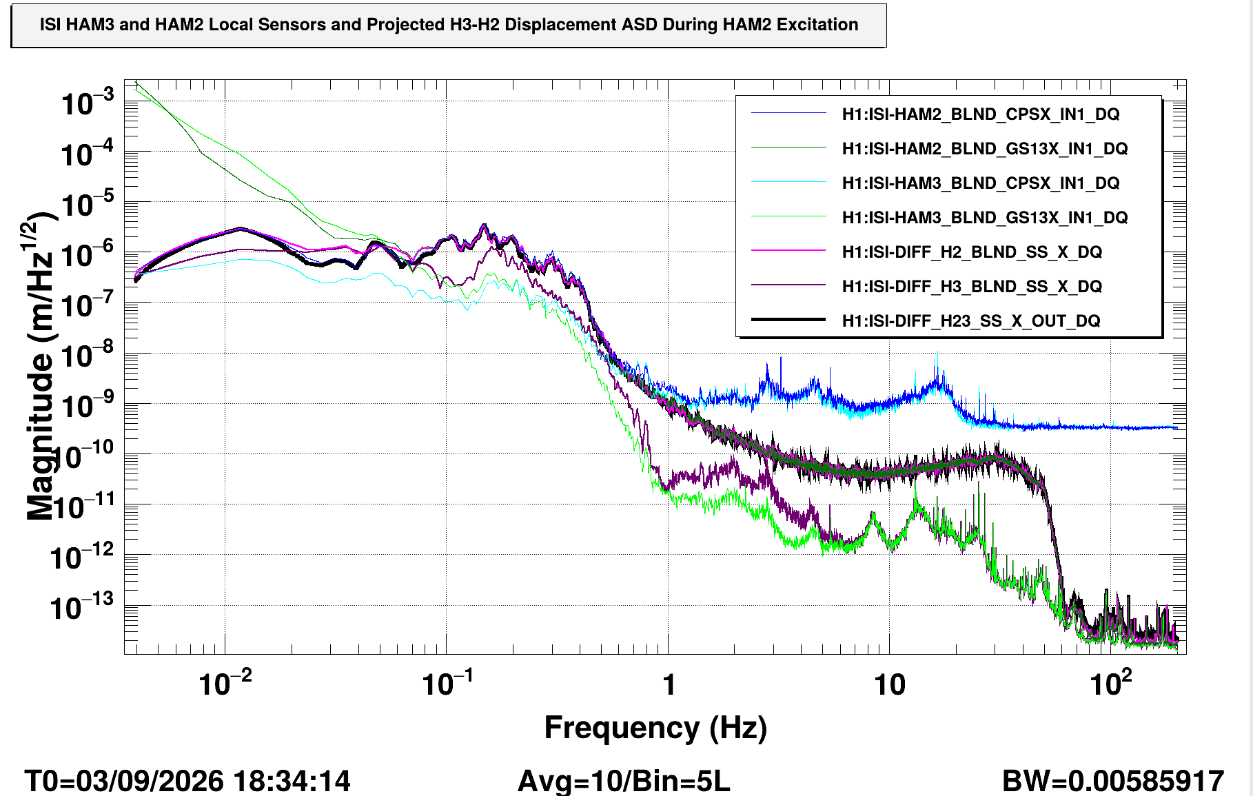
Building up an understanding of the front-end-computed HAM3-HAM2 super sensor signal, H1:ISI-DIFF_H23_SS_X_OUT_DQ.

This ASD collection compares the CPS and GS13s of HAM2 and HAM3 against the differential super sensor during the HAM2 excitation (only). Since HAM3 was NOT being driven, we can treat this like the "reference" performance for the HAM2 ISI -- because the HAM2 and HAM3 ISI typically perform similarly in the longitudinal, or ISI and IFO X direction (when the CRS is not engaged into the HAM3 blend).

- Compare BLUE, DARK GREEN, and HOT PINK traces. We see that the drive on causes displacement on HAM2 is factors of 2x to 50x above the reference level
- Compare THIN DARK PURPLE against CYAN and BRIGHT GREEN traces. We see that the blended input to the super sensor for HAM3 has -- for some reason -- a lot more motion than the "raw" blended CPS and GS13s input.
- COMPARE BLUE, DARK GREEN, HOT PINK, and BLACK traces. Where the CPS and GS13s are not noise limited (i.e. where're signals are used in the blend to form the super sensor sum), All of the HAM2 and the differential HAM3-HAM2 signal agree, showing the excitation on HAM2.

Conclusion: the front-end computed measure of the differential motion between HAM3 - HAM2 using the onboard CPS and GS13s is functional, comes with a calibration that makes sense, and is measuring the right thing.

Attachment 2
Building up more trust in the HAM3-HAM2 super sensor signal, H1:ISI-DIFF_H23_SS_X_OUT_DQ as a faithful signal for comparison with the SPI L signal H1:SPI-H23_DIFFDISP_MAIN_OUT_DQ.

This ASD collection compares the CPS- and GS13-computed differential X motion (BLACK) and SPI L measured differential X motion (RED) during both the reference quiescient time (DASHED traces) and during the HAM2 excitation (SOLID traces). The excitation is also shown (H1:ISI-HAM2-ISO_X_EXC, calibrated into displacement units [m]).

- During the reference time (DASHED), the SPI L and the on-board sensors only agree above 5 [Hz]. *very interesting* We know the low-frequency-end -- below ~2 [Hz] -- is dominated by the SPI seed laser's frequency noise -- which is dominated by the IMC's displacement. Remember, at the time of measurement, only the IMC is locked (but now with the JAC locked between the PSL and IMC). It looks like -- at least during this measurement -- that's larger or different or incoherent with the HAM3-HAM2 motion. So... maybe this is all suspension noise (or ISI tilt)? Needs more study / noise budgeting.

- During the excitation time (SOLID), the SPI L and the on-board sensors agree across a much broader frequency-band, only disagreeing between 1.5 and 10 [Hz]. *very interesting*. *great* that the excitation i.e. this amount of differential motion *makes* the SPI L and on-board sensors agree for the most part. I have even less of a guess at an explanation for the frequency region where they're not, tho.

Conclusion: Under large differential displacement, the SPI L agrees with the on-board sensors over a very broad range of frequencies, from 0.005 - 2 [Hz] and 10 - 60 [Hz] Lots still to investigate, tho.

Attachment 3
Linear transfer function between the HAM3-HAM2 super sensor signal, H1:ISI-DIFF_H23_SS_X_OUT_DQ and the SPI L signal H1:SPI-H23_DIFFDISP_MAIN_OUT_DQ, as well as the length/frequency control channel for the input mode cleaner (H1:IMC-F_OUT_DQ.

I show the driven transfer function magnitude for these signals on a log-log plot. Coherence shown separately below.

- Where the SPI noise didn't match the ISI-DIFF noise between ~2 - 10 [Hz], the TF is incoherent (coherence shown separately below), so ignore that.
- At other frequencies, where the ASD "visually agree" the transfer function is NOT exactly 1.0 -- see more discussion of the values of the TF magnitude in the semilogx version of the plot below. *very interesting*
- I don't understand the magnitude of the IMC-F transfer function at all below 1 [Hz]. The next plot shows it's coherent... *very interesting* or *I'm missing something obvious*

The IMC-F channel has the following calibration into [m]:
    Gain: 1.1683e-06
    Poles: 0
    Zeros: (none)
I don't remember how I calculated this, or where I got it from. To be (re)investigated... but I would have guessed -- since IMC-F_OUT_DQ is already calibrated into [kHz], that it *should* be something like a factor of (2 * L_IMC * lambda / c) = 1.1724e-13 [m/Hz] or 1.1724e-13 [m/kHz] with no poles at 0 [Hz], from df / f0 = dL / L_rt math, but that doesn't seem to be it at all. I probably just need to go back to the code used to produce plots in the SPI final design doc ... just haven't had time.

Also -- side note -- looked into the IMC_X calibration infrastructure that uses the length drive to MC2 to calibrate the control signal into displacement units and that doesn't work.

Attachment 4

Coherence between SPI L and the ISI-DIFF channel and the IMC-F channel for the two TFs shown above.
I also show the coherence between the SPI L channel and the individual ISI CPS and GS13s to understand from where the coherence comes (expecting more from HAM2 since this is during the HAM2 drive.)
I also show the coherence between the ISI-DIFF channel and the IMC just to see how that's different.

Conclusion: Lots to see here, but I haven't really digested it or tried to make sense of it.

Attachment 5
Same transfer function as in Attachment 3, just shown in semi-log x so we can read off what the magnitude of the TF is at coherent frequencies.

- The TF is indeed almost a flat 1.0 [m/m] above 10 Hz; but not quite. *very interesting*
- Between 0.1 and 1 [Hz], where the SPI and ISI-DIFF are *definitely* coherent, the TF magnitude is *not* 1.0, not is it flat. It's got bumps and wiggles between 1.0 and 0.7. Best first guess it that this has something to do with gain peaking in the blend filters. *very interesting*

Conclusion: this TF is going to be very interesting, and we won't be able to "just" blend the SPI "right in" with a simple filter. And, I need to try to get more coherence below 0.1 [Hz].

Very interesting!


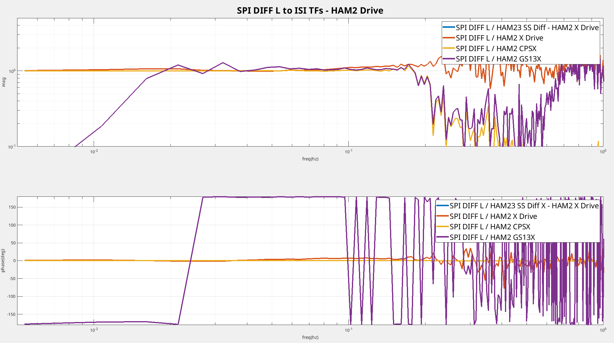
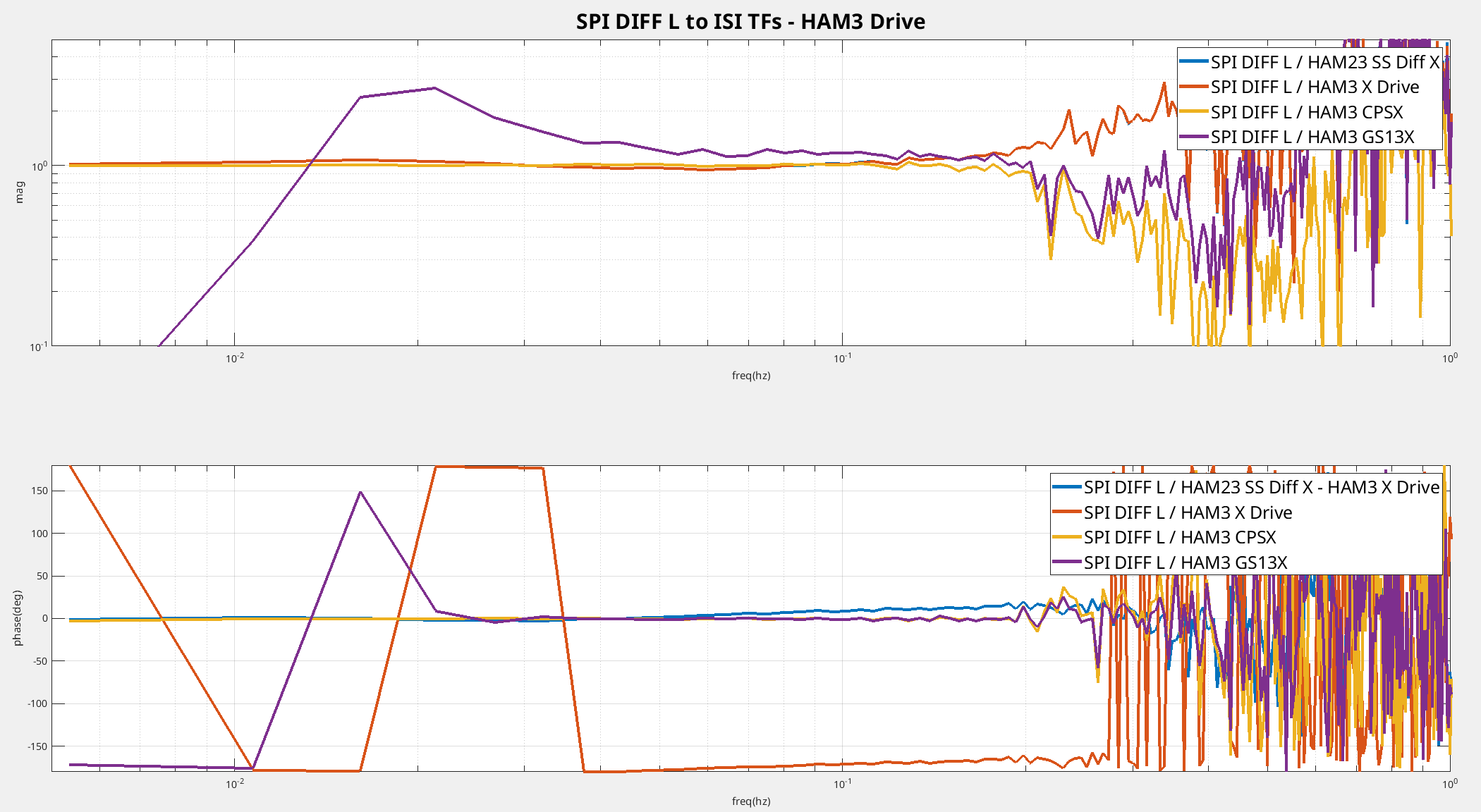
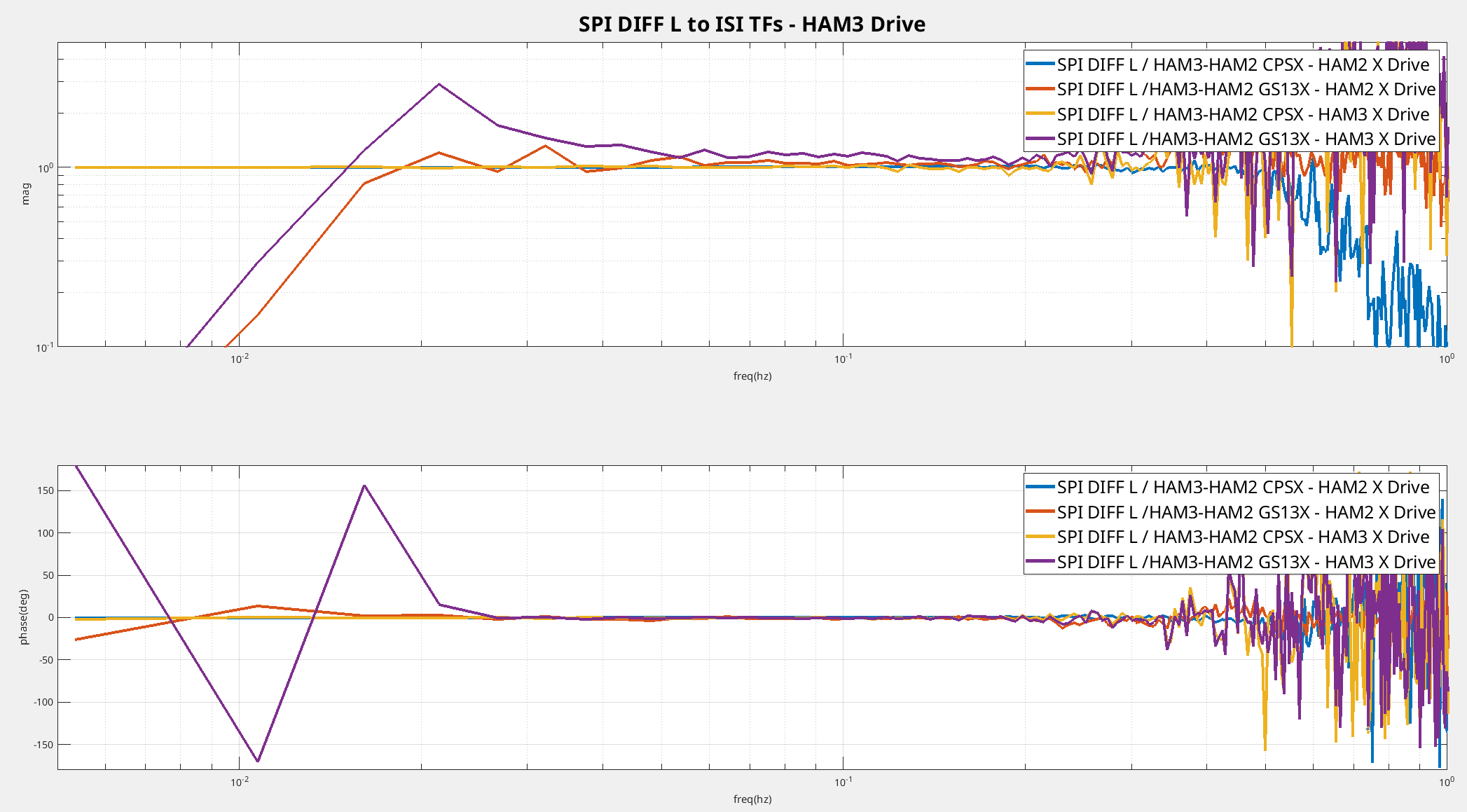
While Jeff was out, I took a somewhat different measurement for SPI differential motion. My excitation was narrower than the one Jeff did here, I just wanted to try to check the calibration at .1hz and below. The first two attached plots are the transfer functions between the SPI DIFF length channel and mostly various ISI sensors. The third image compares the tfs from SPI diff length to differential (HAM3 - HAM2) CPS and GS13s. I'm adding this last plot because I have seen something that looks like the blend filter gain peaking above .1hz in the DIFF SS synthetic supersensor channels, as Jeff mentions above. I think this indicates a drawback to using this synthetic supersensor signals.
For these tfs, it looks like around .1hz the SPI and CPS agree very well, within a percent for my tfs.