TITLE: 06/10 Day Shift: 1430-2330 UTC (0730-1630 PST), all times posted in UTC
STATE of H1: Planned Engineering
OUTGOING OPERATOR: None
CURRENT ENVIRONMENT:
SEI_ENV state: MAINTENANCE
Wind: 11mph Gusts, 5mph 3min avg
Primary useism: 0.04 μm/s
Secondary useism: 0.12 μm/s
QUICK SUMMARY:
SPI Is Shutters and Shutdown, they did not and are not going Laser Haz. So the LVEA remains in LASER SAFE / Bifuircated @ HAM7.
But a lot of work was done for SPI today.
The cable for the TCS Pico drivers was changed out by fil for the SPI team.
Dave wanted to do a DAQ restart for CRS but ran into Model issues and postponed until tomorrow.
Jonathan is restarting some IOCs for Dave and Patrick's work.
HAM2 TF were taken after Fil completed Ground Loop checks.
Alignment of Hepi was blocked by potentially metal on metal touching. Jim is contemplating his options.
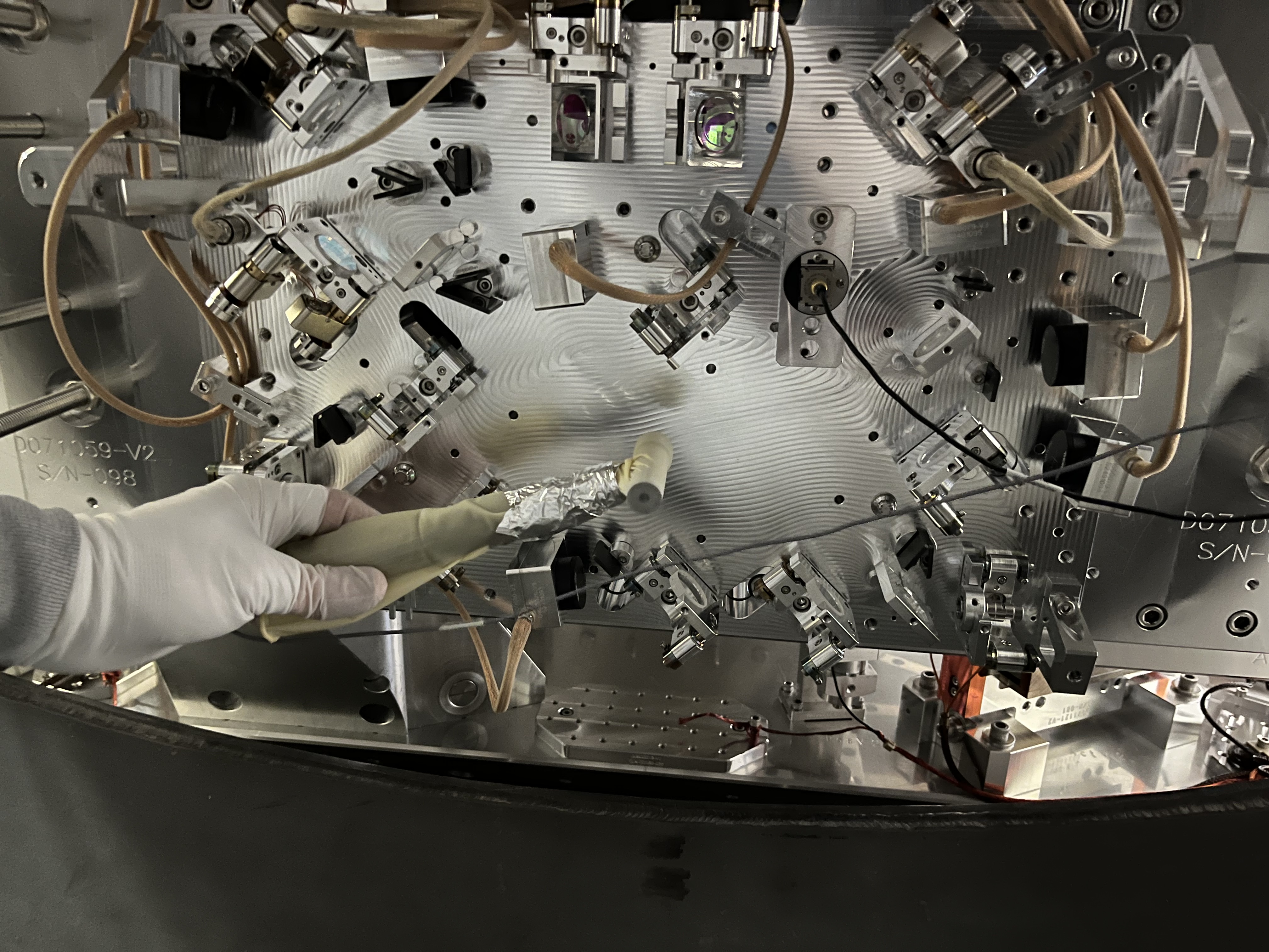
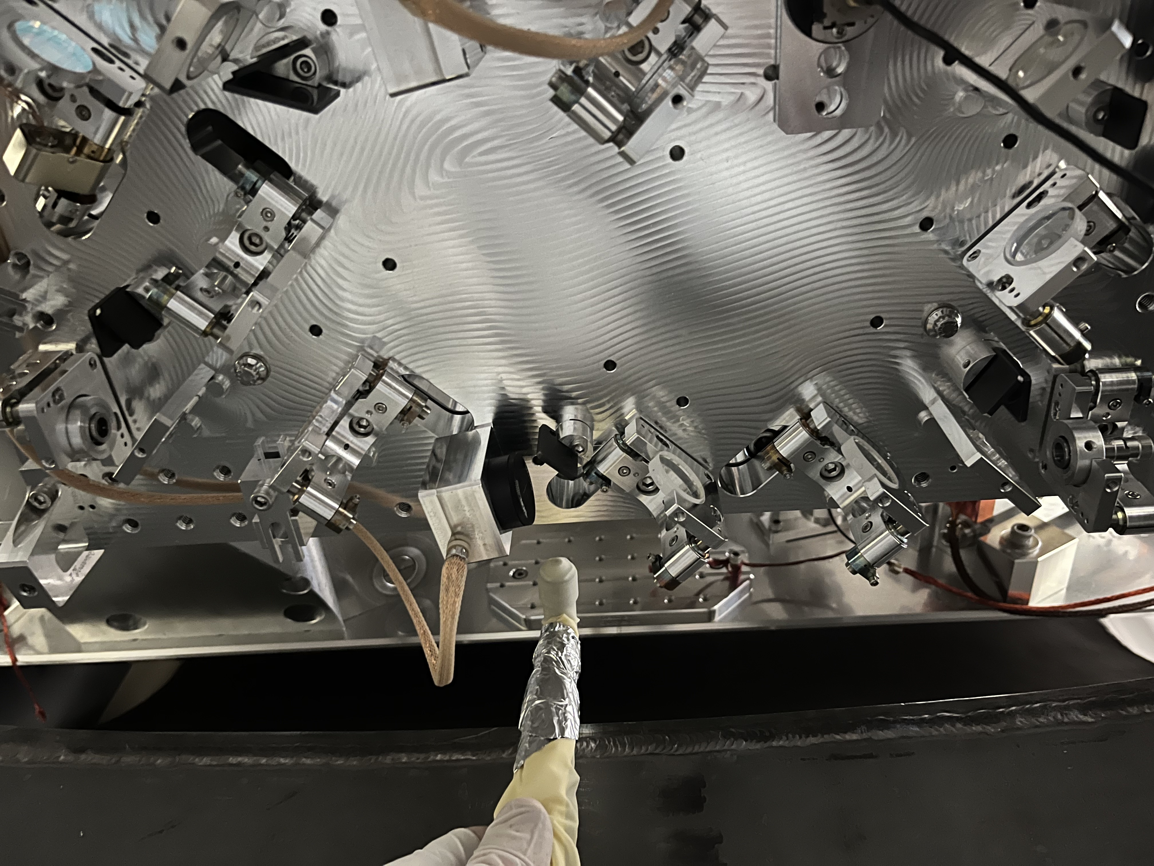
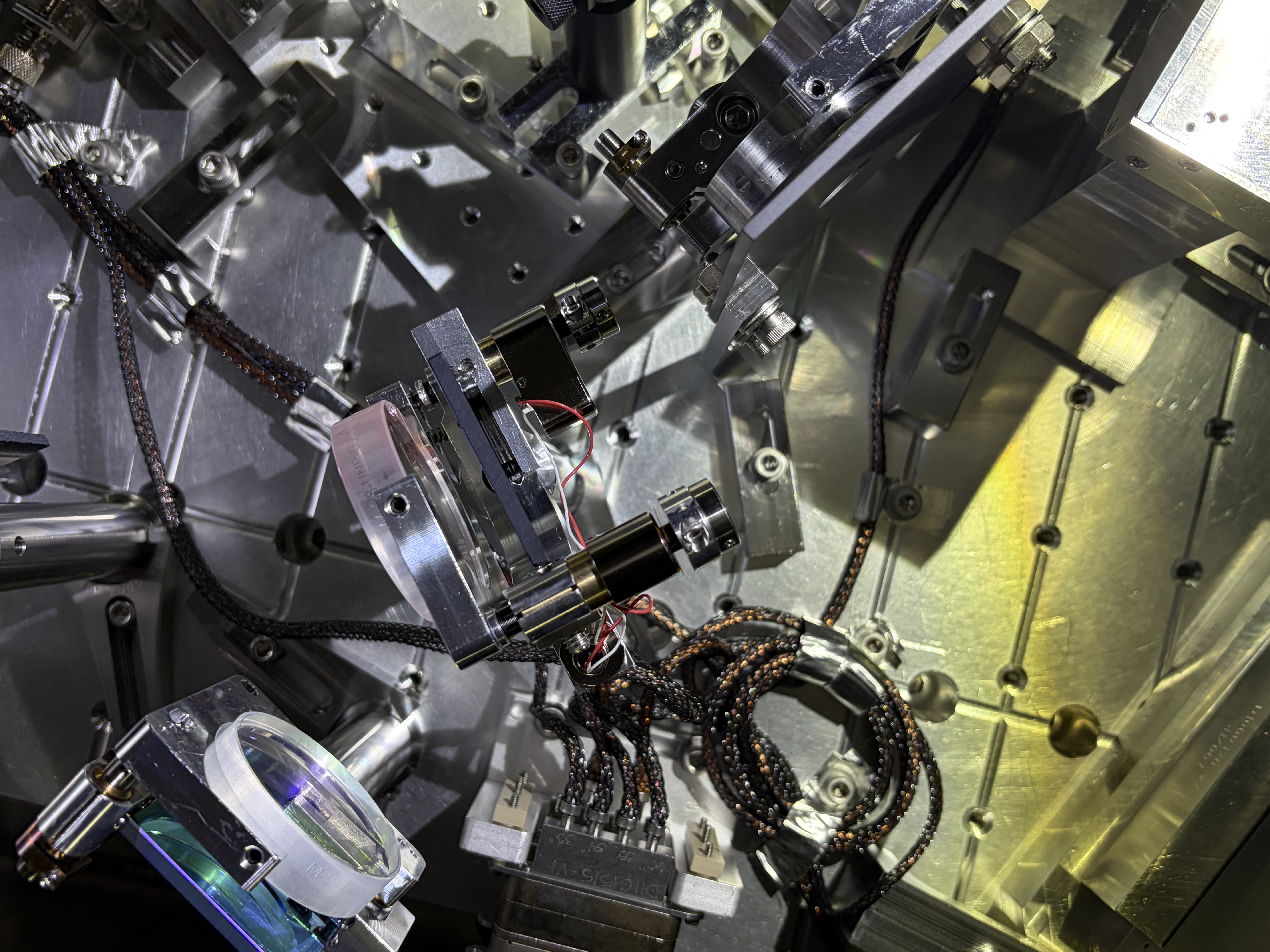
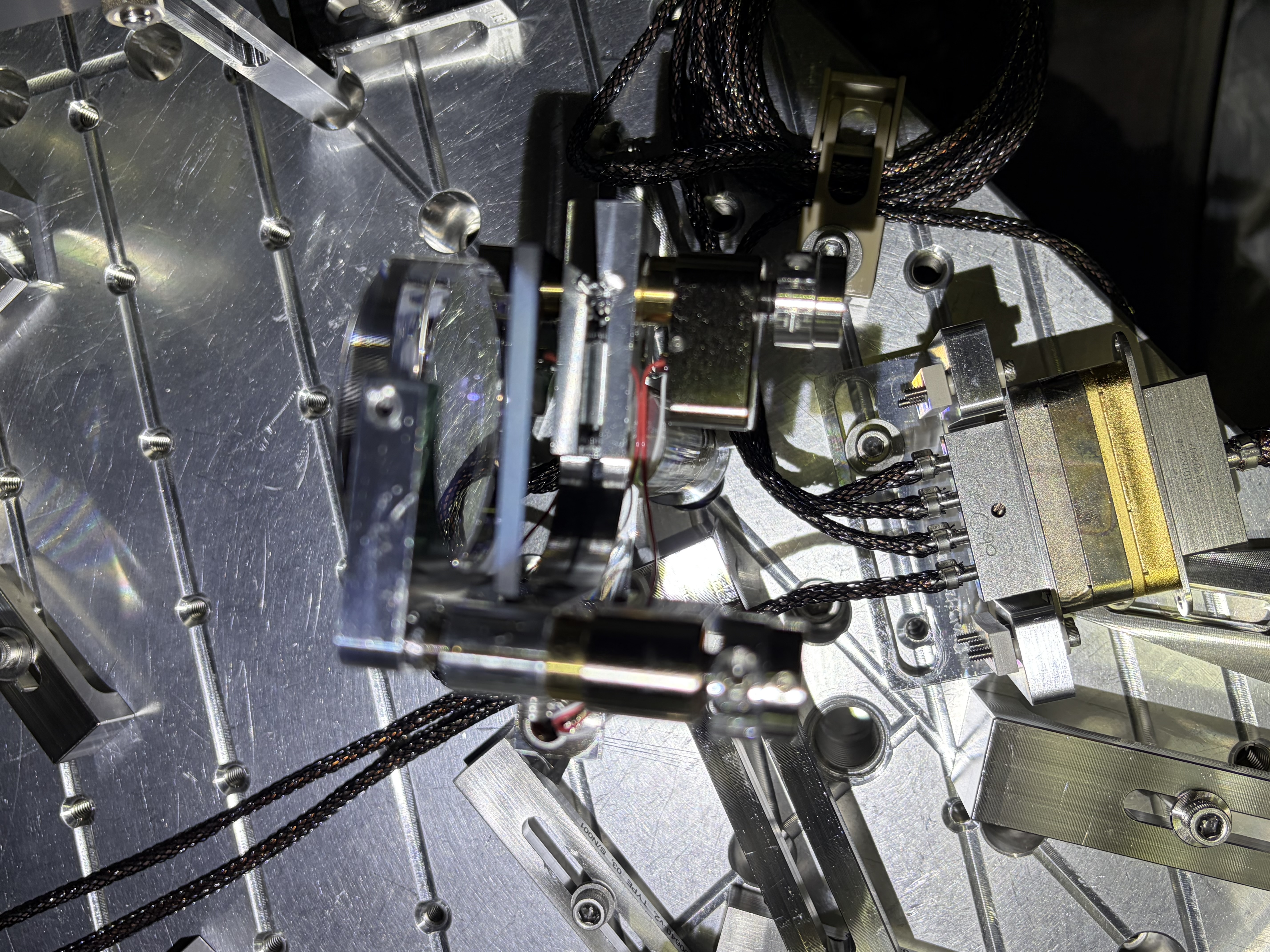
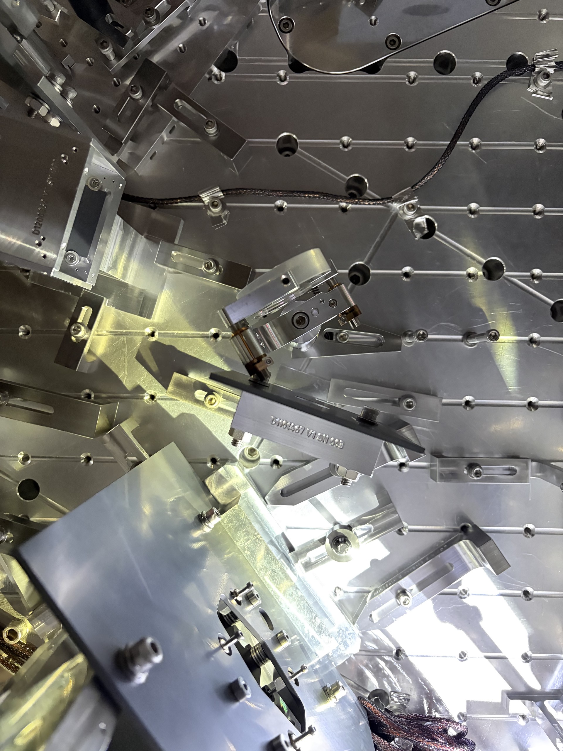
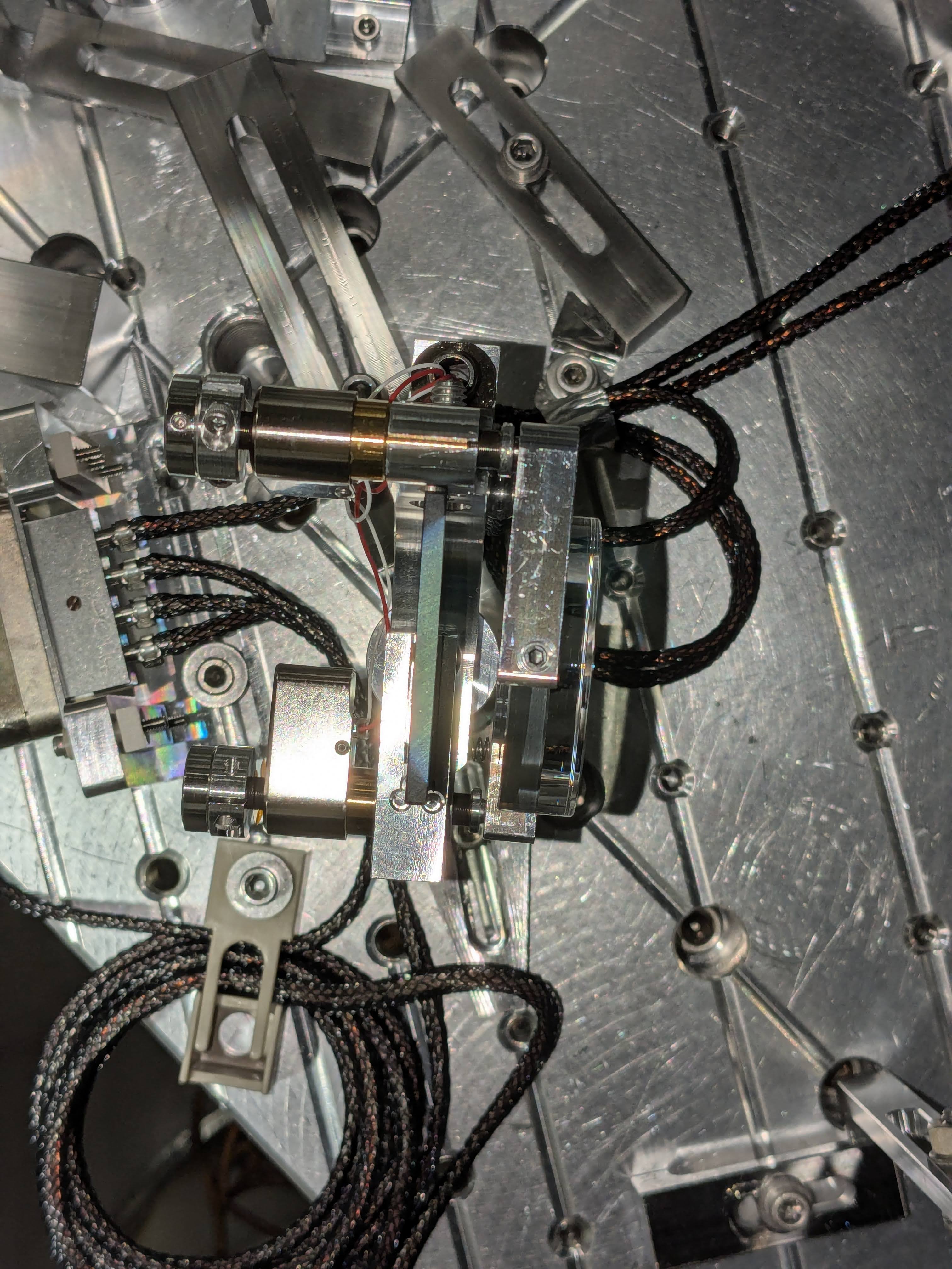
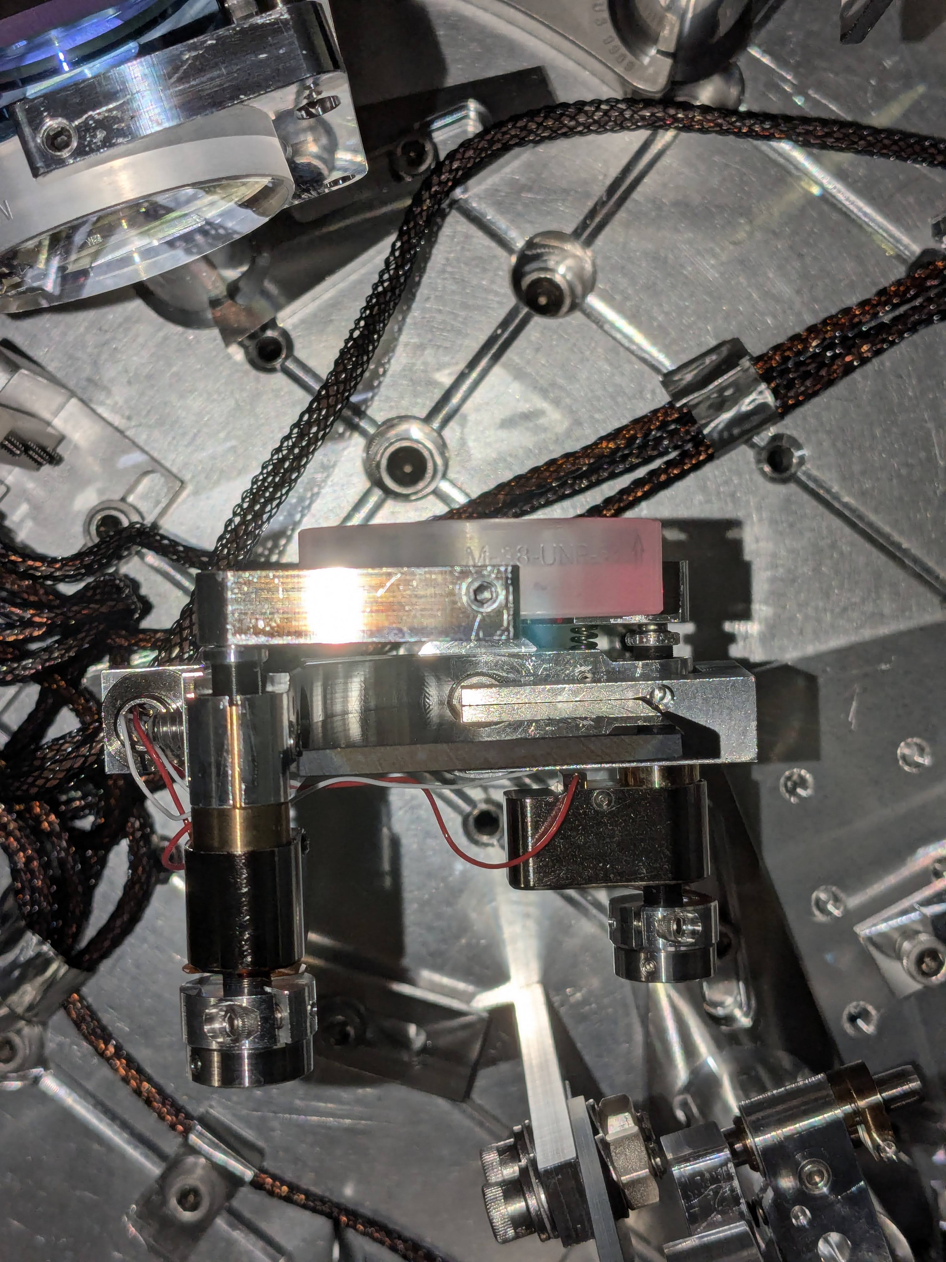
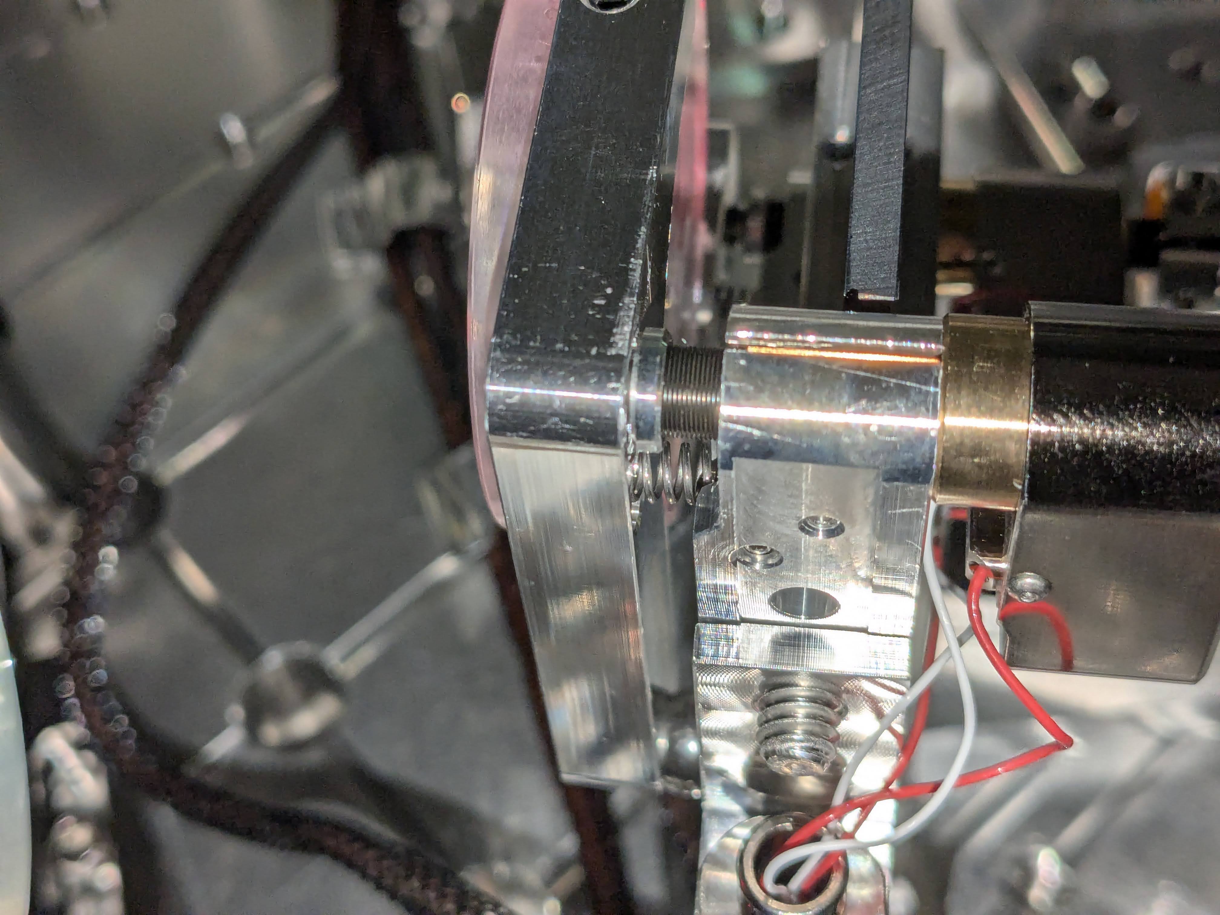
Fist contact of ITMY completed today. Please see tear off in Control room.
GRB-Short E64093 @ 23:46 UTC
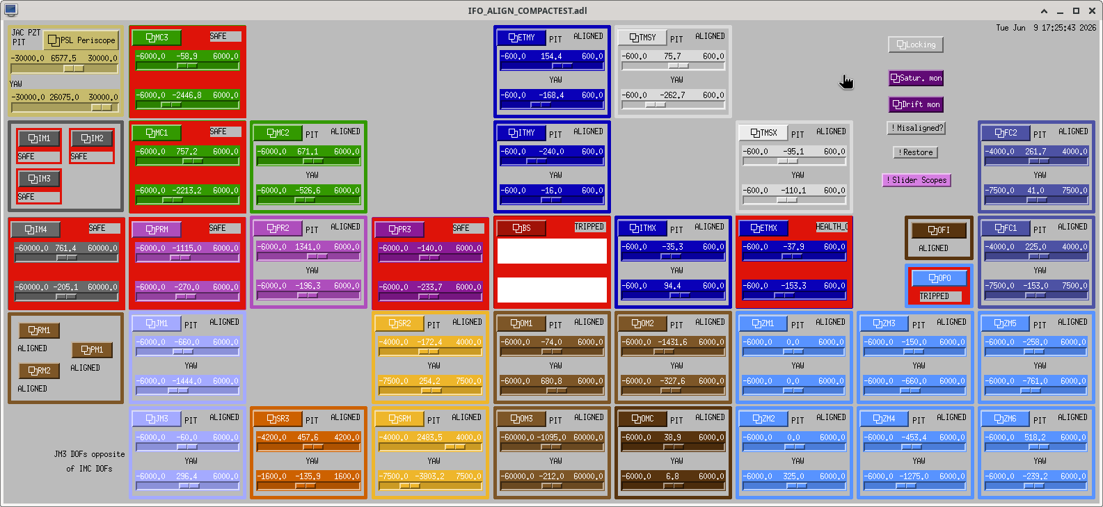
And all the SUS in HAM2 have been set back to Aligned.
| Start Time | System | Name | Location | Lazer_Haz | Task | Time End |
|---|---|---|---|---|---|---|
| 22:52 | SAF | LVEA is Laser SAFE | LVEA | NO | LVEA is Laser SAFE | 16:52 |
| 14:40 | FAC | Kim | LVEA | n | Technical Cleaning & resupply | 15:38 |
| 15:02 | FAC | Randy | LVEA | n | Moving Nitrogen bottle | 15:13 |
| 15:49 | FAC | Kim & Dawn | LVEA | N | technical Cleaning and Resupply | 16:53 |
| 15:59 | IAS | Ryan C | LVEA | N | Warming up the Faro surveying tools | 18:24 |
| 16:14 | SEI | Mitchel | LVEA | N | Helping Jim with BSC2 & HAM2 SEI work | 16:26 |
| 16:35 | SPI | Josh | LVEA | n | SPI install work HAM3 | 19:11 |
| 16:36 | SEI | Jim | LVEA | n | Balance HAM2 ISI | 19:19 |
| 16:36 | IAS | Jason | LVEA | n | FARO HAM3/BSC2 | 18:24 |
| 16:39 | SPI | TJ, Jeff | LVEA | n | B&K SPI breadboard HAM3, TJ out early | 19:18 |
| 16:44 | SUS | RyanS, Anamaria, Ibrahim | LVEA | n | Pulling ITMY first contact in BSC1 | 20:40 |
| 16:45 | EPO | Corey | LVEA | n | Taking photos of first contact pull in BSC1 | 20:39 |
| 16:47 | SPI | Jennie | LVEA | n | SPI install work HAM3 | 18:36 |
| 17:11 | BSC2 | Betsy | LVEA | N | Checking Doors then working on BSC2 | 19:59 |
| 17:19 | SQZ | Camilla & Sheila | LVEA HAM7 | LOCAL | Working in HAM7 | 19:33 |
| 17:22 | SUS | Tom & Alex | Vac Prep | N | Making Cables. | 19:22 |
| 17:53 | EE | Fil | LVEA | N | Ground loop checks. | 14:53 |
| 18:17 | VAC | Travis | LVEA | N | Feed throughs on HAM3 | 20:46 |
| 18:19 | FAC | Kim | HAM Shaq | N | Technical Cleaning & Resupplies | 18:51 |
| 18:42 | SPI | Jennie W | LVEA HAM3 | N | Working on SPI with Josh | 19:11 |
| 18:44 | Safety | Richard | LVEA | N | Chatting with Sheila from across the Bifurcation | 18:53 |
| 19:37 | TSC | Camilla | LVEA TSC cabinets | N | Checking on the TSC cabinets. | 19:47 |
| 19:39 | FAC | Chris & Eric | EY then EX | N | Dropping off new racks | 21:39 |
| 19:59 | SPI | Josh | LVEA | n | Going to SUS R2 rack to test fibers | 23:10 |
| 20:08 | SPI | Jennie W & Jeff | LVEA | N | SPI working call with Sena inside HAM3 | 23:06 |
| 20:09 | SEI | Jim | LVEA | N | HAM2 SEI work | 20:44 |
| 20:15 | SUS | Alex & Tom | Vac Prep | N | making more cables. | 21:36 |
| 21:01 | VAC | Travis | LVEA | N | Cheing the Pump cart | 21:38 |
| 21:14 | SEI | Jim, Ryan, Jason, Mitchel | LVEA | N | Working on BSC2 HEPI alignment , Mitchel Out @ 2230 | 22:36 |
| 21:30 | EE | Betsy & Fil | LVEA HAM2 | N | Rechecking Ground loops andother HAM2 work. | 22:00 |
| 21:31 | SEI | TJ | LVEA BSC2 | N | Helping Jim with HEPI Alignment | 22:29 |
| 21:41 | CDS | Dave | EX | N | scoping and pluging cables & DAQ restarts | 22:14 |
| 21:42 | PEM | Ryan S , Annamaria | LVEA HAM2 | N | Unlockign ITMs and Cleaning up | 23:04 |
| 22:01 | BSC2 | Betsy & Ibrahim | LVEA BSC2 | N | Checking on BSC2 work and cleaning up | 23:33 |
| 22:11 | SQZ | Sheila, Begum, Camilla | LVEA HAM7 | LOCAL | Working on SQZr beam profiling. Sheila out @ 2257 | 23:41 |
| 22:17 | EE | Fil | LVEA SPI & SUS racks | N | Checking cabling connections and grounding. | 23:27 |
| 22:27 | CRS | Alex, S. Apple, | Optics lab | B | Cleaning optics. | 23:40 |
| 22:32 | VAC | Jordan, travis | LVEA | N | Looking for parts. | 22:53 |
| 22:33 | CRS | S.Apple & Oli | LVEA | N | Looking for the Top Gun. | 22:47 |
| 23:11 | CDS | Jonathan | Remote | N | Restarting some IOC | 23:31 |
| 23:38 | SEI | Ryan C, Jason | LVEA BSC2 | N | Inside the BSC2 Chamber. | 00:38 |


