Dave, Jonathan, Tony, operators, ...
This is a compilation of recovery actions based off of a set of notes that Tony took while helping with recovery. This is to augment the already existing log entries 88381 and 88376. Times are localtime.
Thurs 4 Dec
At 12:25 PST power went out. Tony and Jonathan had been working to shut down some of the systems so that they could have a graceful power off. The UPS ran out around 1:17 PST. At 2:02 the power came back.
Tony checked the status of the network switch, making sure they all powered on and we could see traffic flowing.
We started up the DNS/DHCP servers, as well as made sure the FMCS system was coming up.
Then we got access to the management box. We did this with a local console setup.
The first steps were to get file servers up, we needed to get /ligo and /opt/rtcds up. We started on /opt/rtcds as that is what FE computers need. We turned on h1fs0 and made sure it was exporting file systems. H1fs0 was problematic for us. The opt/rtcds file system is a ZFS file system. We think that the box came up, exported the /opt/rtcds path, and then got the zpool ready to use. In the mean time another server came up and wrote to /opt/rtcds. This appears to have happened before the zfs filesystem could be mounted, so it created directories in /opt/rtcds and kept the zfs filesystem (which had the full contents of /opt/rtcds) from mounting. When we noticed this we deleted the /opt/rtcds contents on h1fs0, made sure the zfs file system mounted, and then re-exporting things. This gave all the systems a populated /opt/rtcs. We had to reboot everything that had started as they ended up now having stale file handles. There were still problems with the mount. The file system performance was very slow over nfs. Direct disk access was fast when testing on the file server. We fixed this the next day after rulling out network conjestion and errors.
We then turned on the h1daq*0 machines to make it possible to start recording data. However they would need a reboot to clear issues with /opt/rtcds, and would need front end systems up in order to have data to collect.
Then we went to get /ligo started. We logged onto cdsfs2. As a reminder cdsfs2,3,4,5 are a distributed system with the files. We don't start this much so we had forgotten how. Our notes hinted at it. Dan Moraru helped here. What we had to do was to tell pacemaker (pcs) to leave maintenance mode, then it started the cdsfsligo ip address. Dan did a zpool reopen to fix zfs errors. Then we restarted the nfs-server service. At this point we had a /ligo file system. We updated the notes on cdswiki as well so that we a reminder for next time. The system was placed back into maintenance mode (the failover is problematic).
The next step was to get the boot server running. This was h1vmboot5-5, that lived on h1hypervisor. This is a kvm based system, that does not use proxmox, like our vm cluster. So it took us a moment to get on, we ended up going in via the console and doing a virsh start on h1vmboot5-5.
Dave started front-ends at this point. Operators were checking the IOC for power.
We started the 0 leg of the daq.
We started the procmox cluster up and began starting ldap and other core services. To get the VMs to start we had to do some work on cdsfs0 as the VM images are stored on a share there. This was an unmount of the share, starting zfs on cdsfs0 and a remount.
Ldap came up around 4:31. This allowed users to start logging into systems as themselves.
Turned on the following vms
- ldapmgmt
- ldaprep1
- ldaprep2
- extalert
- cdsioc0
- beckhoffimages
- cdsioc1
- condamirror
- h0epics
- epicsburt
- seismon2
- Note we should get rid of seismon and seismon1 vms
We powered on the epics gateway machine.
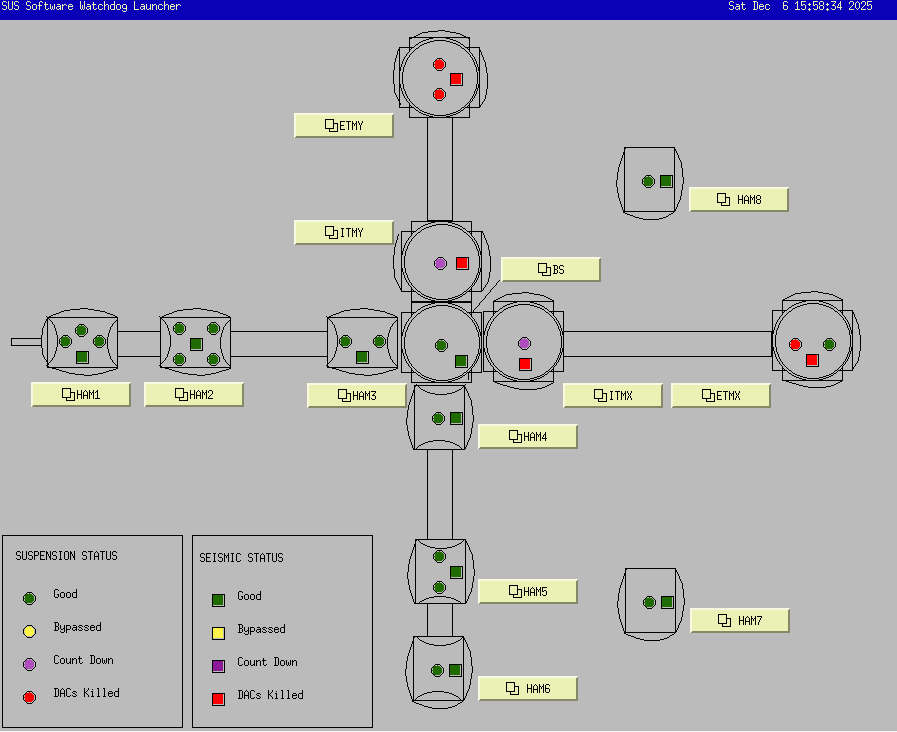
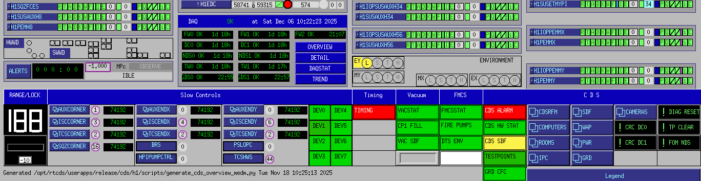
We needed to reboot h1daqscript0 to get mounts right and to start the daqstat ioc. This was around 5pm. The overview showed that TW1 was down. We needed to bring and interface up on h1daqdc1 and start a cds_xmit process so that data would flow to TW1. We got TW1 working around 5:15pm.
Powered on h1xegw0, and fmcs-epics. Note with fmcs-epics the button doesn't work (it is a mac mini with a rack mount kit), you need to go the back and find the power button there.
Reviewing systems, we turned off the old h1boot1 (there are no network connections, so it doesn't break anything to power on, but it should be cleaned up). Powered on the ldasgw0,1 machines so that h1daqnds could mount the raw trend archive.
The epics gateways did not start automatically, so we went onto cdsegw0 around 5:45 and ran the startup procedure.
The wap controller did not come up. Something is electrically wrong (maybe a failed power supply).
At 6:01 Dave powered down susey for Fil. It was brought back around 6:11.
Through this Dave was working on starting models. The /opt/rtcds was very slow and models would time out while reading the safe.snap files. Eventually Dave got things going.
Patrick, Tony, and Jonathan did some work on the cameras while Dave was restarting systems. We picked a camera, cycled the network switch port to power cycle the camera. Then restarted the camera service. However this did not result in a video stream.
Friday
Jonathan found a few strange traffic flows while looking for slow downs. These were not enough to cause the slow downs we had. h1daqgds1 did not have it's broadcast interface come up and was transmitting the 1s frames out over its main interface and through to the router. So this was disabled until it could be looked at. The dolphin manager was sending more traffic to all daqd boxes trying to establish the health of the dolphin fabric. It was not a complete fabric as dc0 was not brought back up as it isn't doing anything at this point. In response we started dc0 to remove another source of abnormal traffic from the network.
These were not enought to explain the slow downs. Further inspection showed that there was not abnormal traffic going to/from h1fs0 and that other than the above noted traffic there was no unexpected traffic on the switch.
It was determined the slow downs were strictly nfs related. We changed cdsws33 to get /opt/rtcds from h1fs1. This was done to test the impact of restarting the file server. After testing restarts with h1fs1 and cdsws33 we stopped the zfs-share service on h1fs0 (so there would not be competing nfs servers) and restarted nfs-kernel-server. In general no restarts where required, access just returned to normal speed for anything touching /opt/rtcds.
After this, TJ restarted the guardian machine to try and put it into a better state. All nodes came up except one, which he then restarted.
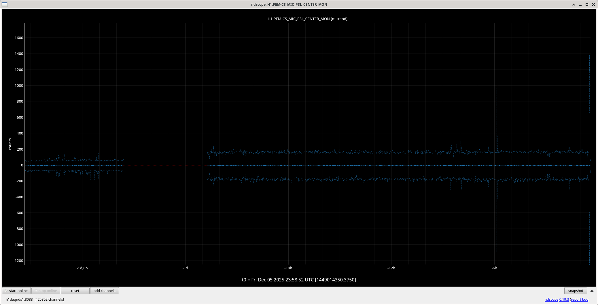
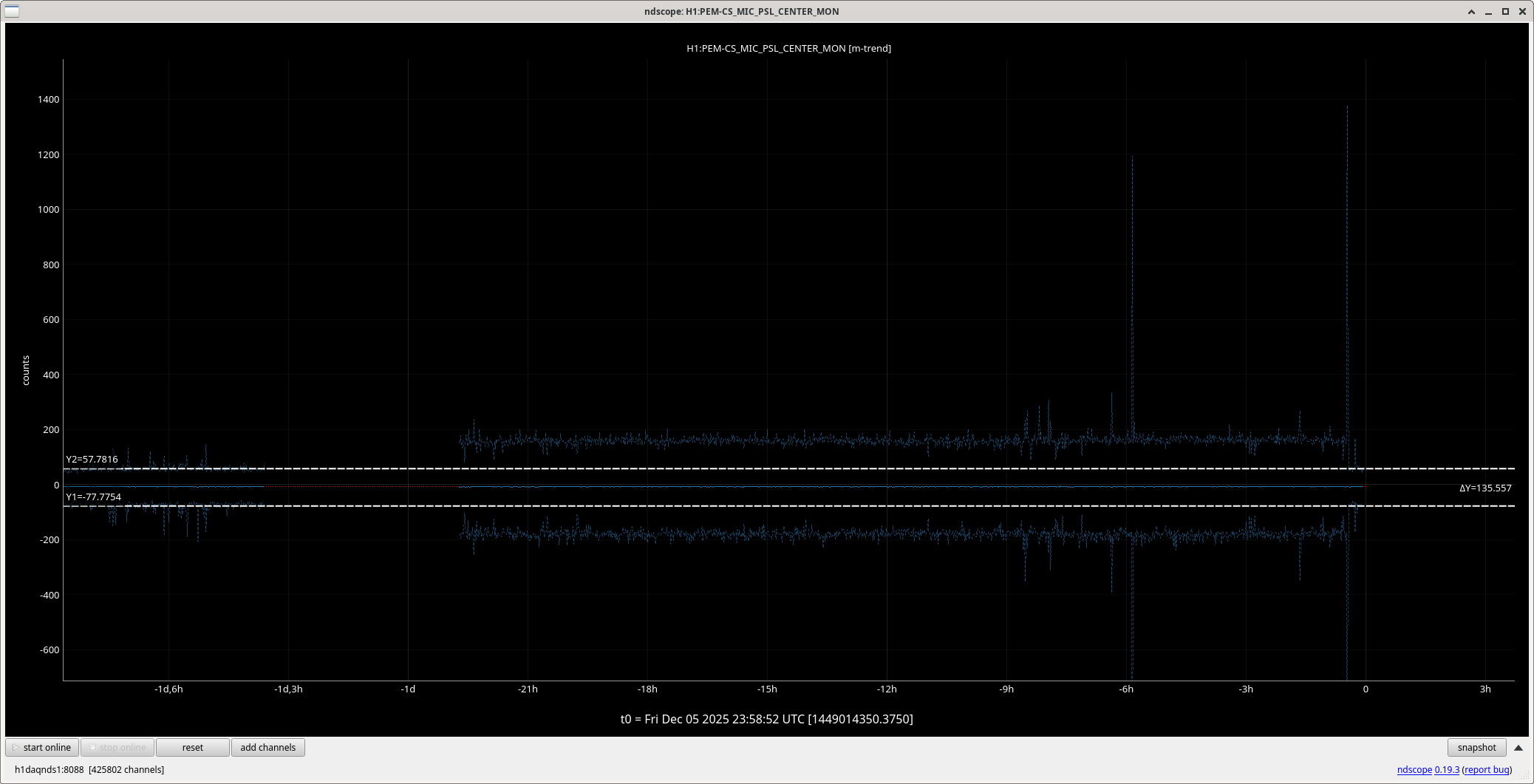
Dave restarted h1pemmx, which had been problematic.
We restarted h1digivideo2,4,5,6. This brought all the cameras back.
Looking at the h1daqgds machines the broadcast interface had not come back. So starting the enp7s0f1 interfaces and restarting the daqd fixed its transmission problems. The 1s frames are flowing to DMT. At Dan's request Jonathan took a look at a DMT issue after starting h1dmt1,2,3. the /gds-h1 share was not mounted on h1dmtlogin, so nagios checks were failing due to not have that data available.
The wap control was momentarily brought to life. It's cmos battery was dead so it needed intervention to boot and needed a new date/time. However it froze while saving settings.
The external medm was not working. Looking at the console for lhoepics, its cmos battery had failed as well and needed intervention to boot.
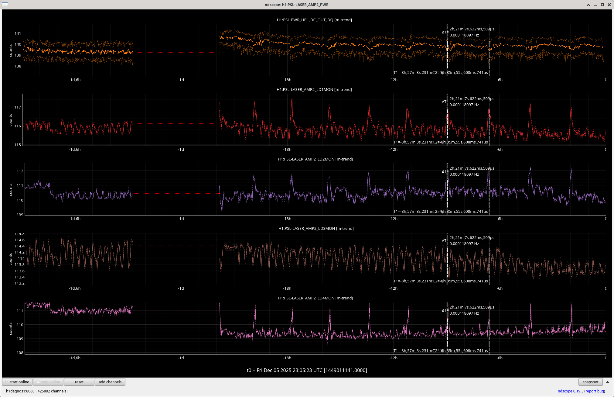
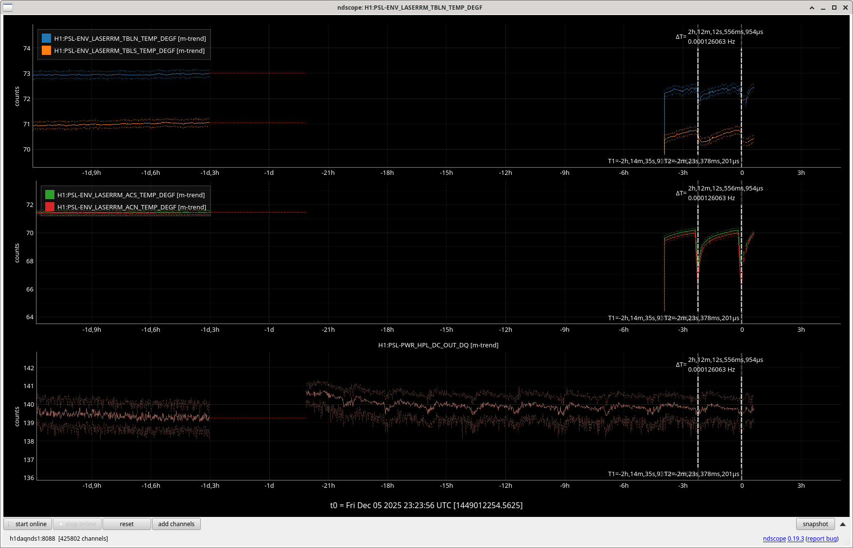
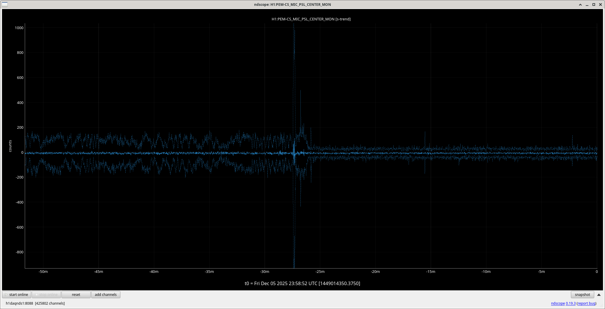
After starting ldasgw0,1 yesterday we were able to mount the raw minute trend archive to the nds servers.
Fw2 needed a reboot to reset it's /opt/rtcds.
We also brought up more of the test stand today to allow Ryan Crouch and Rahul to work on the sustriple in the staging building.
A note, things using kerberos for authentication are going slower. We are not sure why. We have reached out to the LIAM group for help.