Addressed TCS Chillers (Wed [Jun3] 713-726am local time) & CLOSED FAMIS #64381.   It's been a while since this has been checked due to issues with FAMIS for LHO.

For measurements below, measuring from "top" of the red floaty ball.

• TCSx Chiller:  Had level of 28.5 cm.  Added 270mL for 30.6cm.
• TCSy Chiller:  Had level of 9.0 cm.  Added 475mL for 10.5cm.  
• There was no water in the small cup under the slow leak.

TITLE: 06/03 Day Shift: 1430-2330 UTC (0730-1630 PST), all times posted in UTC
STATE of H1: Planned Engineering
OUTGOING OPERATOR: None
CURRENT ENVIRONMENT:
    SEI_ENV state: MAINTENANCE
    Wind: 5mph Gusts, 2mph 3min avg
    Primary useism: 0.02 μm/s
    Secondary useism: 0.12 μm/s 
QUICK SUMMARY:

• HAM2 work continues
• HAM3, cabling, SPI install?
• ITM cage baffling continues

J. Kissel, S. Koehlenbeck, J. Wright, P. Opperman

After the most of the day Monday (2026-06-01) ruling out of the prime suspect (the picomotors causing alignment drift; see LHO:90438), I left discouraged that we had ruled our everything that could be spatially wrong with the MEAS beam going into the MEAS IFO (power, alignment, mode-shape, and polarization). However, Sina and special-guest consultant Patrick spent time reviewing everything that we ruled out and/or what it could be -- and Sina left the lab nudging the NPRO seed laser's crystal temperature from 24.6 [deg C] to 25.2 [deg C].

%%%%%%%%%%%%%%%
Executive Summary: Nudging the NPRO seed laser by 0.6 [deg C] (we believe) changed the resonant mode in the laser, stabilizing its output frequency. (We believe) the laser was in-some-way frequency drifting and/or mode hoping (a thing that would also be driven by the clean room environment in the ways we suspected were impacting the transceiver), and the path length differences between the REF and MEAS IFOs were discrepant enough (per the design layout) that the efficiency impact was much larger on the MEAS IFO. Having adjusted the laser crystal temperature, both IFOs are stable for hours and if/when small drift is seen its common to both IFOs as the gods intended. We can't claim we 100% understand it, or believe our own story, but it worked!

Finally happy with both the MEAS and REF IFOs, we mounted the transceiver vertically and confirmed its function in that orientation.

We're a go for install, and have started to dissect the production equipment from the optics lab.
%%%%%%%%%%%%%%%

Some victory photos attached.

Other things that happened:
    - Prior to laser temp adjustment -- with MEAS IFO path on fully manually driven mounts -- we foiled (as protection) then C3 covered (as isolation) the transceiver. We still saw drift. That put the nail in the coffin that it wasn't transceiver itself that was sensitive to the environment.
    - We re-installed all picomotor-driven IXM100 mounts to support M_M1, M_B4, and M_M2.
    - Prior to install, we were able to (rather barbarically) back off stopper nuts of the pitch picomotors for the M_B4 and M_M2, so there is no longer any question whether the stopper nut is driving moving plate. All pitch and yaw actuators push the moving plate kinematically via the intended ball-bearing-to-carbide-plate design.
    - Re-installed M_M4 M_M5 periscope mirror mounts, including their adapters and D1800200 Type 07 beam-dumps. The dumps were parked in a position that still allowed transmission of the MEAS beam (as confirmed with no change in the -- now stable! -- MEAS IFO efficiency).
    - Nudged IFO MEAS A and IFO REF A PDs because the beam spot on the diodes was a bit OFF.
    - Reviewed and confirmed all PD reflected beams were on their respective dump, except for the known issue with the FBR_PWRIN_REF PD that reflects 0.2 [mW] of power up above the breadboard.
    - Built up a temporary vertical mounting system with 1 [inch] posts and small cylindrical laser holding mounts with mini bread-board feet.
    - Re-installed the handles on ISIK.
    - Unbolted, and was easily able to single-person lift the entire assembly and mount it.
    - Both IFO efficiencies were actually not-that-bad after installing. Wow!
    - A quick alignment tune-up from Sina recovered all the IFO efficiency we had while mounted horizontally. 
    - Both IFOs were stable and happy for the entire series of victory photos we took; about 1 hr.

Camilla, Betsy, TJ, Fil, Ryan C, Richard, Erik, Dave

We had a very strange problem with the first 20bit-DAC in h1sush7, which h1susfc1 uses for its six M1 drives (T1, T2, T3, LF, RT, SD). Even though h1iopsush7 reported that DAC0 was driving correctly, there was no voltages being produced by the AI chassis.

We are in the early stages of figuring out what was wrong and how it got fixed. Due to HAM7 in-chamber urgency, once it started working we handed h1sush7 over the the HAM7 team.

Summary of what we did is:

tried various power cycles of IO Chassis and AI Chassis, no change. Put DVM onto DAC cable at rear of AI Chassis, looking at CH0 initially. No voltage. IOP correctly detected loss of AI.

With IO Chassis powered up, but computer down, Fil saw 3.5V on CH0, which went to 0V as soon as the computer was powered up. We are not sure this is normal behaviour, but we saw it on two different 20bit-DAC cards. 

Next we replaced the 20bit-DAC, no change. Old (removed) 210303-09 New (installed) 210303-14.

Erik reminded us that since this is the first DAC in the IO Chassis, we can test CH7 with the DUOTONE loop back (IOP feeds ADC0-CH31 directly into DAC0-7, switches relays on Interface cards which routes DAC0-7 into ADC0-30). We turned this on, ADC0-30 saw the DT. 

Next we replaced the DAC's ribbon cable and interface card. This make things worse, no CH0 signal and now no Duotone. Interface old (removed) S1101353, new (installed) S1000868.

Thinking that ribbon cables are more likely to fail than IF cards, we went back to the original IF card S1101353, installed another ribbon cable, and shuffled DAC0 over to the second Adnaco backplane. THIS FIXED IT.

Several changes were made here, so we are not sure if it was the slot move or the ribbon cable or both.

Here is the original card layout (not shown A4-1 = BIO0)

and here is the one we ended up with (ADCs shuffled one left in A2, 20DAC0 moved to A2-1)

We tested the first 6 channels (CH0-CH5) using h1susfc1 by untripping the watchdogs and driving the DAC with a FM offset of 10000, resulting in a 20bit-DAC drive of ~40000 counts, which gives 0.7V DAC output. CH7 was tested with the Duotone.

I was reminded that on the 1st December 2025 the h1iscex 18bit-DAC to 20bit-DAC upgrade failed with no drive on the new DAC. That was also the first DAC, and at the time we tested the DUOTONE signal (in fact DAC-DT is always on for CAL). In that DAC all the channels were not operational, and replacing the DAC fixed it immediately. So it looks like today's problem is different, and a much more insideous one because internally everything looks nominal but no voltage is actually sent by the DAC.

Shoshana, Alexandra, Jim, Arnaud

Today we completed the build of x4 HOQIs (D2500104), wired the capacitive plates of two CRS (following pinout from D2500389, with cap A = Left plate and cap B = Right plate), and hung one CRS with a dummy flexure.

Tomorrow we will align and tune the HOQIs, and hung the CRS with its final flexure.

A few things to note:
*We used undersize (0.0625" for 0.063" hole) dowel pins on the baseplate to set the alignment of the 4 BS cubes, then removed the pins from underneath the plate. While this was our plan B, it worked quite well (initial design was to use 1/16" spring pins, but they are hard to insert without bending them). 
*Some baseplates holes for the dog clamps were not threaded all the way through, we had to use washers to reduce the screw travel range. We will have to order a 4-40 tap and retap those holes.
*Some photodiodes cracked from screwing the setscrew in the holder (but we have enough spares). Details in the HOQI PD Testing tab of the spreadsheet attached to E2400153.
*For next time, we should make sure the photodiode vent hole is not aligned with the setscrew holding the photodiode in place (maybe update drawings D2600047)
*The waveplate holders were scribed with 4 lines for the 1/4 waveplate and 2 lines for the 1/2 waveplate so we can recognize them

Jonathan, Patrick, Erik, Dave:

We restarted the DAQ + EDC around 16:00 this afternoon primarily to install Patrick's new H1EPICS_HEPIPUMPL0.ini to match his new IOC.

At the same time we removed the end station VEA2 Dust monitor channels, there hasn't been a second dust monitor at the ends for some time and the Sat power outage required an EY Dust restart which removed its VEA2 channels from the ioc. We also made the EX INI change for when its IOC is restarted.

To green up the EDC, we temporarily removed h1susbs' FEC-31 channels. Erik has put H1EPICS_[FEC,SDF].ini under puppet control, so these will be added back when h1susbs is reinstalled.

We also fixed an issue whereby yesterday puppet added some incorrect KC0 channels to the EDC. This was fixed today and there are now no KC0 channel in H1EPICS_DAQ.ini, they all reside in the hand-built H1EPICS_DAQKC0.ini. Around today's restart time KC0 coincidently went unstable, restarting itself every 5 seconds. The problem was downstream of KC0. Jonathan contacted LDAS and the problem was fixed within the hour.

The EDC is green again, first time since the power outage.

Good thing:

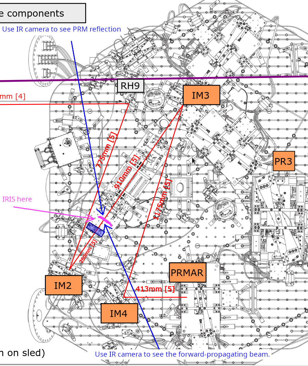
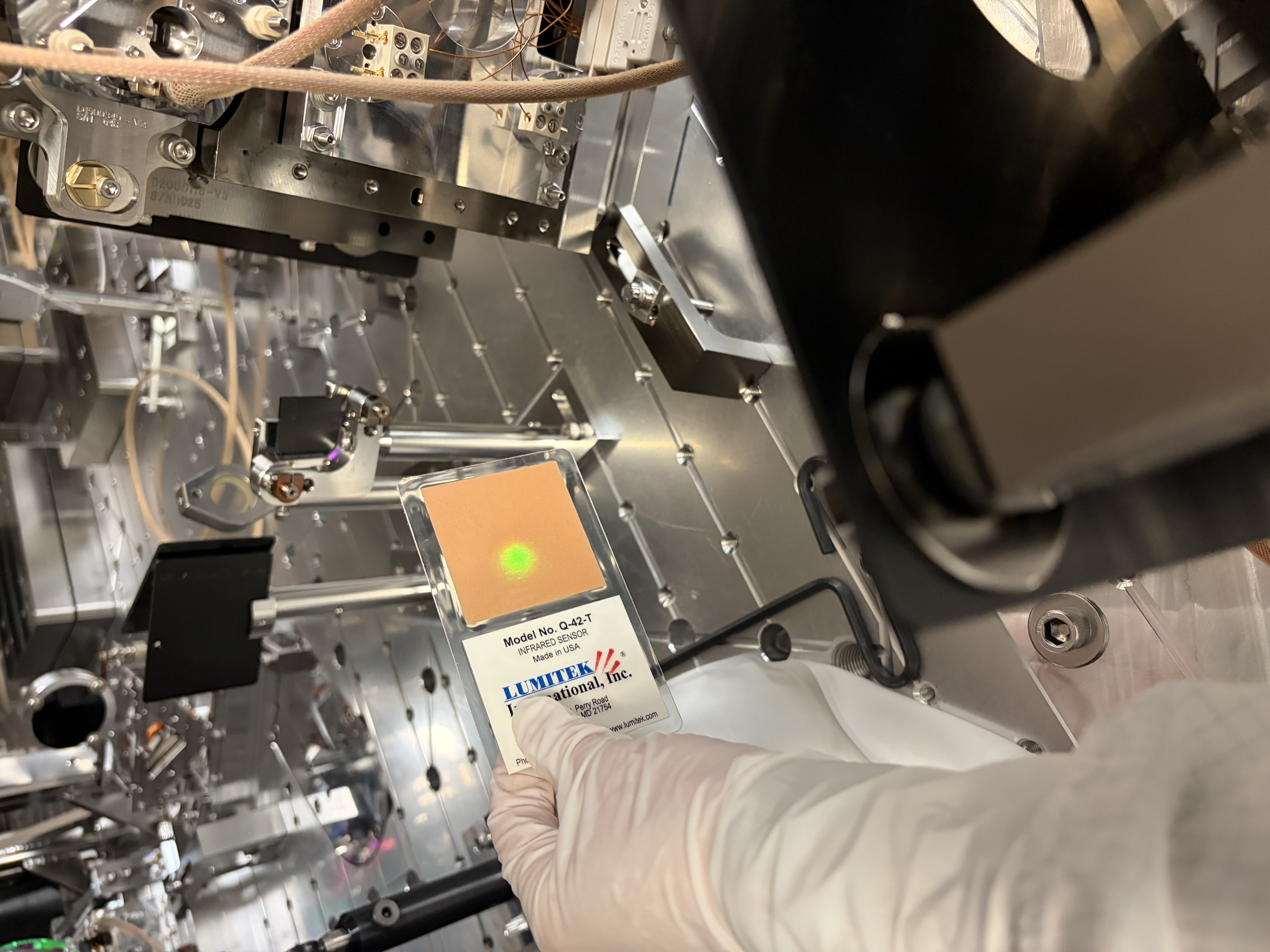
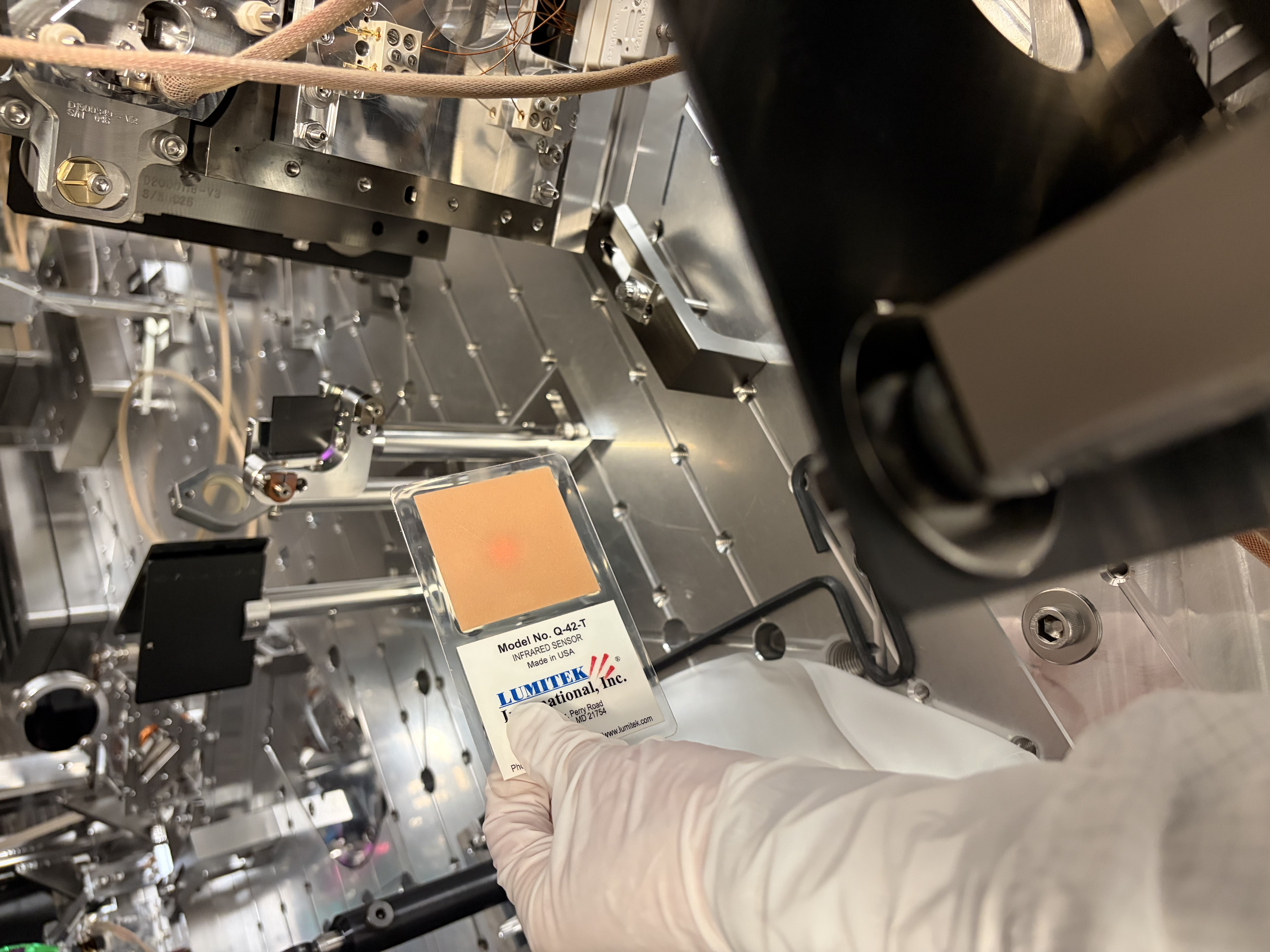
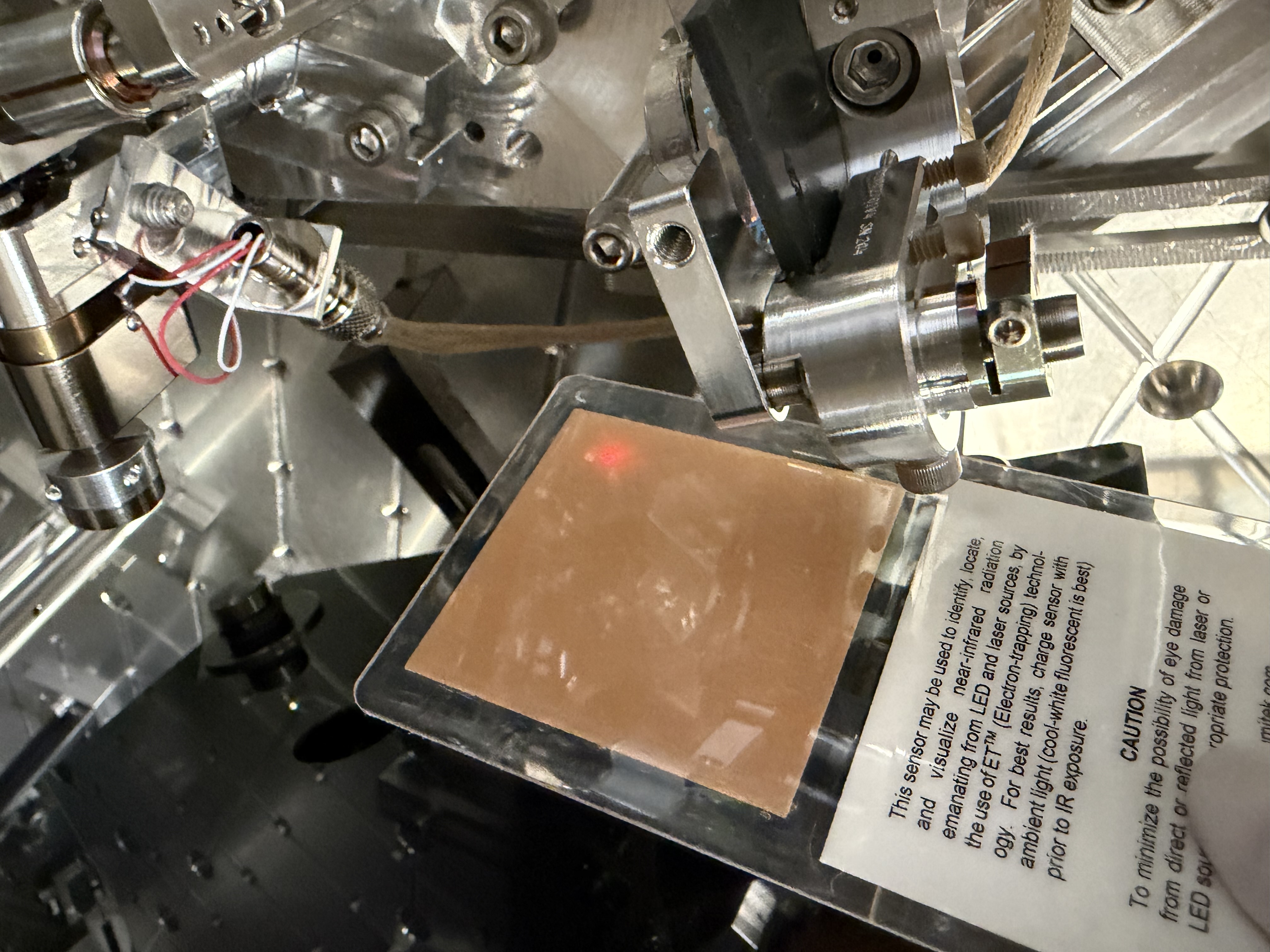
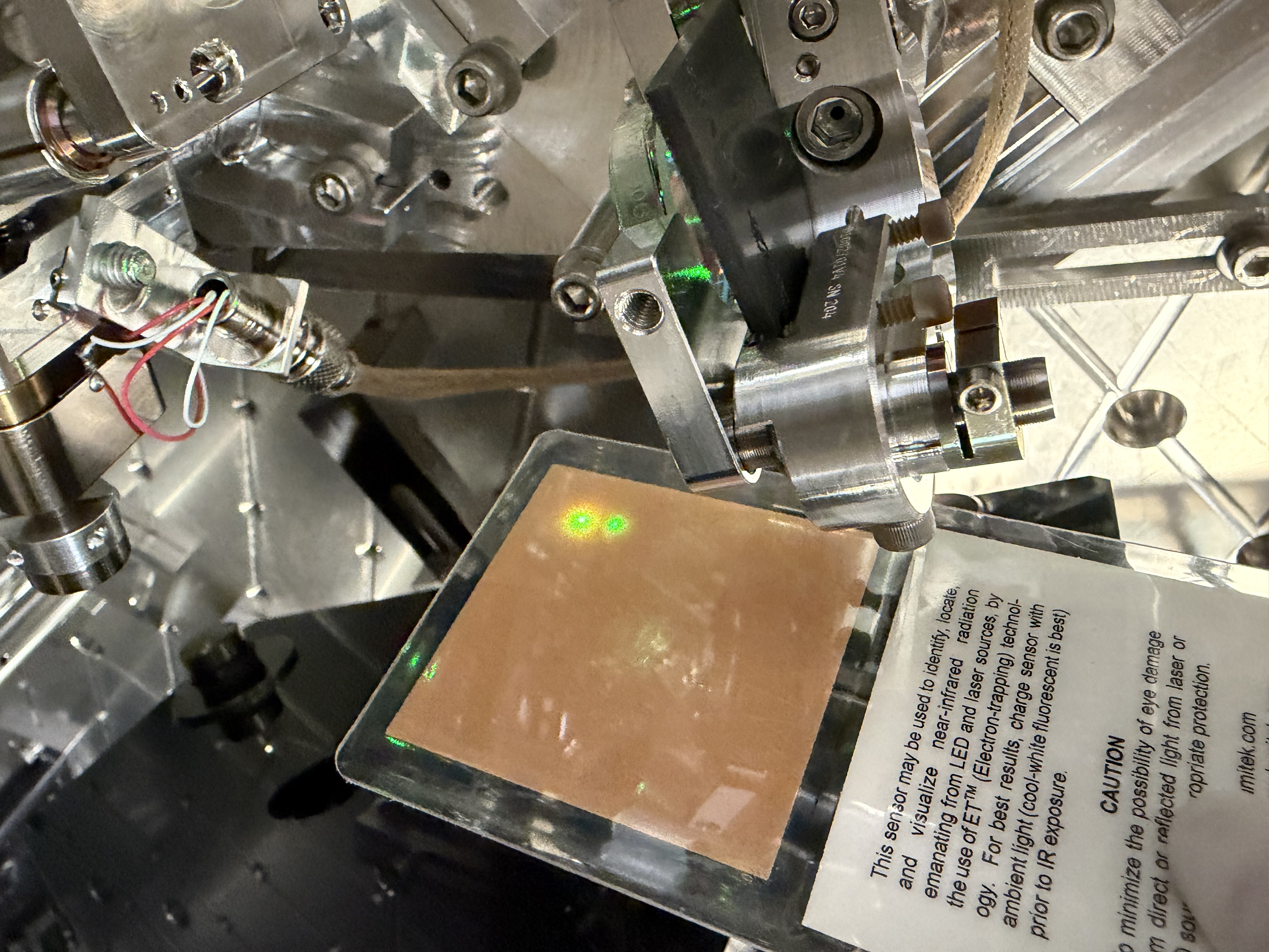
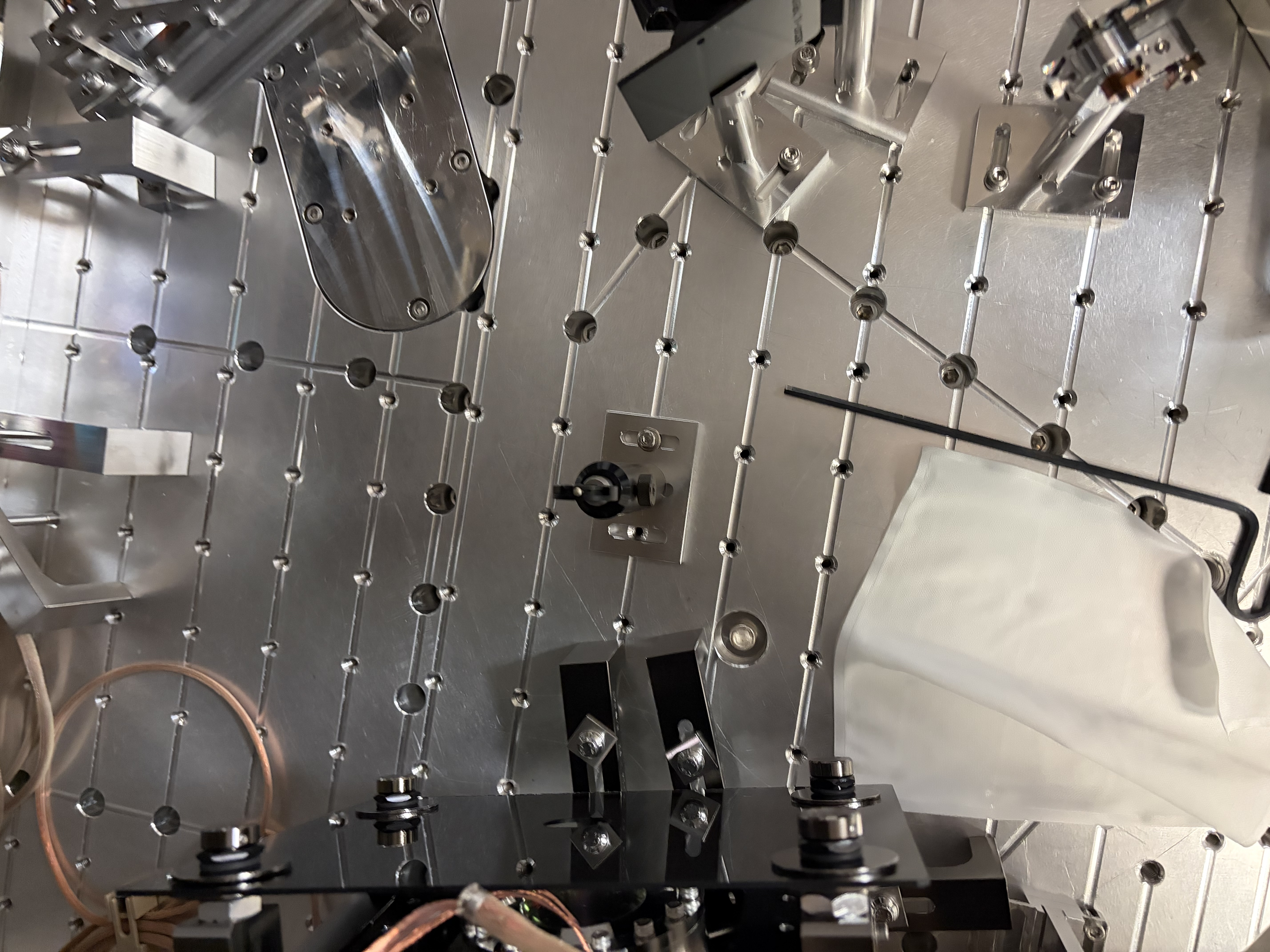
In the morning, we placed an iris placed between the IFI input baffle and the IFI HWP baffle (irisposition.png). We used an IR sensitive DSLR as a viewer to center the iris for the forward-going beam, and observed the back side of the iris using the same camera to see the PRM reflection.

This allowed us to set the PRM angle in much better accuracy than using a card with a bigger-than-needed hole handheld at an inconvenient location and observe with naked eyes through the laser glasses. We had to close down HAM3 cover as well as one side of HAM2 so PRM quiets down, but the retro-reflection accuracy was like +-50 urad (rather than +-500urad of yesterday).

With this new PRM alignment ([P, Y]=[-1165, +750]), I was able to center REFL sensors despite that RM2 was so close to railing, RM2 YAW offset was -1800urad. (ASC_REFL_balanced_20260602_morning.png and ASC_REFL_balanced_but_RM2_close_to_railing_20260602_morning.png.)

Nice thing was, at this point the beam was much closer to the center of IFI input baffle, IFO REFL beam clipping-like thing observed on the IFI input baffle was completely gone as well as the clipping on IM4 baffle. So things looked better in general than they were yesterday.

Bad thing:

RM2 was so uncomfortably close to railing nobody should leave it like that before pumping down, so I decided to relieve RM2 by tilting IM1. (Calculation is in alog 90404.)

I thought RM2 should be rotated counter-clockwise seen from the top because that would mean the positive YAW offset, we added negative 100urad to IM1 YAW offset (i.e. from -887.1 to -987.1 urad) based on my calculation, expecting to shave off 300 or 400 urad from the RM2 YAW. We reset the iris position for the forward-going beam, then reset the PRM angle, fully opened the iris and started centering the REFL sensors. Disappointingly, we couldn't center them, RM2 railed.

What was wrong:

We wasted some time trying to somehow find a magic slider values for RMs and going through how the angle of IM1 propagates to RMs, but it turns out that RM alignment sliders seem to have the opposite sign than all other suspensions. As far as we believe that the OSEM sensor (not actuator) produces positive DAC output that is proportional to the number of photons, the conclusion is that the sign of the sliders is wrong for both RM1 and RM2.

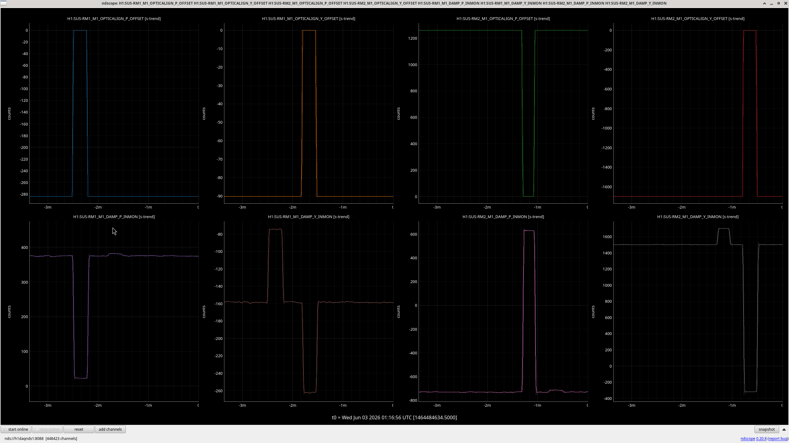
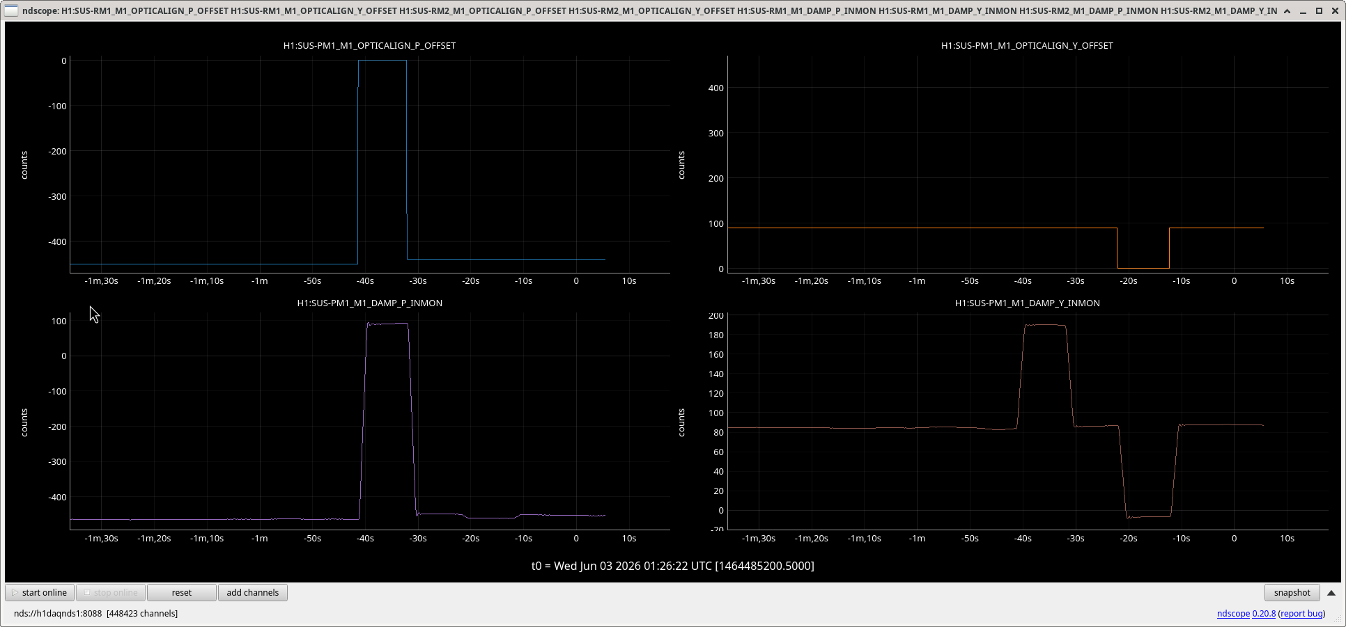
This is clearly shown in wrongsign.png where slider offsets of RMs were zero-ed one by one (top row) while the OSEM sensors in Euler bassis (bottom) were observed. Ignore the cross coupling from P actuation to Y sensing. In a suspension that follows the LIGO sign convention, the slider and the sensors move in the same direction roughly by the same amount. RM is the opposite of that, sensors move in the opposite direction of the sliders. We have done the same test for RMs, PM1 (see PM_is_good.png), OM1 (because they're all tip-tilts) and IM1 (because we touched it today) and confirmed that RMs are an exception.

If you're not sure about the rotation convention of LIGO optics, positive YAW rotation means counter-clockwise seen from the top. This will increase the light power on RIGHT OSEM sensors and decrease it on the LEFT. Given that the ADC reports positive voltage (i.e. positive counts), and given that usually OSEM YAW signal is proportional to voltage(RIGHT)-voltage(LEFT), positive physical YAW rotation will produce positive OSEM YAW change.  See my cartoon (LIGO_YAW_sign_convention.jpg).

Now, RM1, RM2 and PM1 sensing look identical to me (osemsensors_look_good.png).

All OSEMs produce positive numbers for all three suspensions, there's no sign flip in the filters, filter output sign is only determined by whether or not the input is bigger or smaller than the mid-point offset, they all use identical OSEM2EULER matrix as well as SENSALIGN matrix, and the sign of DAMP_P as well as DAMP_Y are all according to the filter outputs and these matrices. So the sensors for RM1 and RM2 are working in the same way as PM1, they're fine.

The conclusion to me is that somehow the actuation sign is wrong for RM1 and RM2.

Rahul told me that the magnet polarity was wrong for RM1 or RM2 and people spent some time to address that issue. But that sounds like the actuation side issue which should NOT affect the validity of the sensors. Unless people tell me that somehow the physical UL/UR/LL/LR sensors are wired to the LR/LL/UR/Ul channel or something, we just believe the OSEM sensors and assume that the sign of sliders is flipped.

Tomorrow:

Regardless of the reason of the sign flip, we'll proceed to move IM1 in the opposite direction, i.e. somewhere between this morning and Friday. 

FYI below is the history of IM1 YAW offset in the past week. The change made on Monday was motivated by the "need" to relieve RM2, but now that we know that the PRM retroreflection accuracy matters, I'm not sure if it would have been impossible to center REFL ASC sensors on Friday if we used the iris technique to align PRM. 

Sheila, Begum, Camilla, Fil, Dave, Erik

Day 2 of the HAM7 work, follow on from 90426. The CDS/EE team fixed the FC1 top mass, unsure how. We found we then could not trust the sliders at all. We reverted all optics (apart from FC1) to the 90183  time. We tired putting the FC1 M3 WIT back to this time but the beam clipped on the OPOS.

Then we moved FC1 to center the IR on the SQZT7 irises. Got perfectly centered on far iris, a little high on iris at the bottom of the periscope.

Begum and Sheila then moved the ZM4 iris to mark this alignment.

TITLE: 06/02 Day Shift: 1430-2330 UTC (0730-1630 PST), all times posted in UTC
STATE of H1: Planned Engineering
INCOMING OPERATOR: None
SHIFT SUMMARY: HAM3 FAROing finished, HAM2, BBS, and SPI work continue. The LVEA is in LASER HAZARD.
LOG:

• FC1 issues were investigated (FRS38162) and fixed.
• 19:53 UTC sush7 restart
• 21:15 UTC Transition to LASER SAFE for Jim to lock ITMX ISI then back to HAZARD
• 22:50-23:05 UTC Periodically I saw seeing red blocks flashing around the COIL OUTPUT FILTER boxes on M0 and M1 for ITMY, I'm guess this was from the crew installing baffles making the osems angry.

Jennie Wright

Summary: Started debugging JAC WFS, two corrections made in WFS segment -> euler basis matrix.

Not sure if this change was made by the power outage or it has been set up wrong the whole time but the channels for segment 3 and 4 in the Q phase matrix for both JAC WFS QPDs were wrong.

This meant yaw = + segment 1 - segment 2 + segment 3 - segment 4 which would be some kind of weird pringle mode.

I corrected the sign, and also updated the note at the bottom right of the JAC_WFS_SETTINGS screen to reflect the sign that the WFS should have (the previous note here described the IMC WFS euler basis as I had copied the medm screen from the IMC custom screens).

now yaw = +1 -2 -3 + 4.

NB: JAC WFS euler basis matches other ASC QPDs but the IMC has P & Y swapped due to the persicopes in HAM2 and so has yaw = +1 + 2 -3 -4 and pitch = +1 -2 -3 +4.

New values for Q matrices are accepted in sdf, as is the PSL PZT mirror offset values that align the beam to the JAC as this has changed since it was last set before the power outage.

Summary: The QOSEMs on the BBSS will see a vertical sag of ~50um. The LF and RT QOSEMs should be offset 50um low of center in there x axis, and the F1, F2, F3, SD QOSEMs should be offset 50um low of center in there y axis; such that they will be well centered when under vacuum.

In T2600176 (write up to come) we calculate the expected vertical sag of the BBSS suspension chain to be 58um at M1. This is slightly larger than the 50um predicted for the BSFM (T1100616), which is consistent with the fact the payload is lighter. To verify these calculations, we pulled OSEM data from the last pump down of the BSFM (April 26 2025 = 1428872333)), and see that there was a vertical sag on the LF and RT BOSEMs of ~35um. See the figure attached.

This is about 10um less than predicted by the calculations for the BSFM, a trend which is also seen on the Quads (LHO alog 15887). As such we suggest that the BBSS should have its M1 QOSEMs offset by ~50um low of center, also about 10um less than the theoretical value. The M2 and M3 OSEMs do not need to be offset, as they don't measure in the vertical direction.

A. Effler, R. Schofield, R. Short

This morning, we started working in BSC1 to prep for the new cage baffle installation on ITMY. Before going into any chambers, Anamaria and Robert moved ITMY to center the OpLev signals. Once at BSC1, Anamaria and I were in the chamber while Robert handled tools in and out as well as kept an eye on particle counts. We started by attaching the long locker bracket on the arm cavity baffle (ACB), then pushed the ACB up and away from the quad after undoing the hinge assembly. While holding the ACB up, we inserted and screwed in the wedge that keeps the ACB away from the quad. With this out of the way, we locked down the bottom two stages of both the main and reaction chains of ITMY by pushing in the earthquake stops until they just came into contact. We then went about replacing the stops on the HR surface of the ITM. After this, we realized that we meant to get measurements of the test mass and reaction mass before they were locked down, so we unlocked the bottom stages of each chain so they were free hanging and took measurements, then re-locked the stages. At this point, we stopped for lunch.

Ibrahim, Tom, Oli

Yesterday we were able to take our first set of transfer functions with the QOSEMs! They are looking good. The measurement files can be found in /ligo/svncommon/SusSVN/sus/trunk/BBSS/H1/BS/SAGM1/Data/2026-06-01_1700/2026-06-01_1700_H1SUSBS_M1_WhiteNoise_{L,T,V,R,P,Y}_0p02to50Hz.xml. I have committed the data files to svn as r13024, but I have not yet exported them or analyzed them in matlab because I want to make sure I do it the same way that LLO has decided to do it.

Tom, Ibrahim, Oli

Yesterday we made a lot of progress on the BBSS, specifically on the QOSEMs.

First, we went around between all the QOSEMs and worked on centering in the X and Y directions. Once we got everything within +/-1000 counts, we made sure the cam adjusters were all tightened. We did this with the constant current switched ON for all the QOSEMs at the satamp, and with the whitening OFF on the satamp but had the compensation ON in medm.

Then we left and were ready to try damping and transfer functions.

We switched the constant current OFF for the QOSEMs now, since we wanted the satamp to be able to adjust the currrent to keep it the same. We also ended up needing to turn the whitening compensation OFF in the model to be able to see the actual amount of movement since it had also been OFF at the satamp.

While trying to damp, we found that we needed to swap the sign of the damping gains to get damping to work. We believe this is because these QOSEM coils, which were made out of older BOSEMs, had the opposite wires from normal connected up, leading to the current flowing the opposite way than expected.

We also needed to lower some of the damping gains.

I've attached a screenshot of how our damping filter bank looks now, but it seems to be working well!

Yesterday I made some changes to the h1suslo12 model(before, after). We were now done with the BOSEMs on the BBSS, so we needed the BBSS model to be able to drive to the DAC for M1 so we could test the QOSEMs. We also needed to be able to switch the BIO on the BBSS, so we also needed to connect the BIO senders and receivers back up to be able to communicate with MC2, which controls the BIO switching for the b2h34 models.

To be able to run this updated model, we would also need to stop the h1susbs model so there wouldn't be mulitple sets of channels trying to write to the same DAC.

Erik and Jonathan (90422) helped with stopping h1susbs, and with building and restarting h1suslo12.

TITLE: 06/02 Day Shift: 1430-2330 UTC (0730-1630 PST), all times posted in UTC
STATE of H1: Planned Engineering
OUTGOING OPERATOR: None
CURRENT ENVIRONMENT:
    SEI_ENV state: MAINTENANCE
    Wind: 8mph Gusts, 4mph 3min avg
    Primary useism: 0.02 μm/s
    Secondary useism: 0.14 μm/s 
QUICK SUMMARY:

• FAROing on HAM3, HAM2 work, and HAM7 continues
• DAQ_KCO channels are disconnected

Sheila, Camilla, Disha

After Jim locked the ISI, Marc bypassed the high voltage interlock, and Camilla restored the psams, we reset the alignment sliders following 90483 which was in air.   The dither locking worked without any issue, and we saw that the beam was low on both the irises in the homodyne path on SQZT7.  Camilla adjusted the alignments of ZM4+ZM5 to center the beam on the irses, screenshot attached shows the alignment that she found.  

We placed an iris in front of ZM4 for this alignment, we were able to look from the +X side of the chamber to check the centering.  We also took photos of the IR/green co-alignment, it looks good coming right off the VIP, but looking right after ZM3 you can see that there is a small misalignment in yaw.  We will continue with placing irses tomorow.