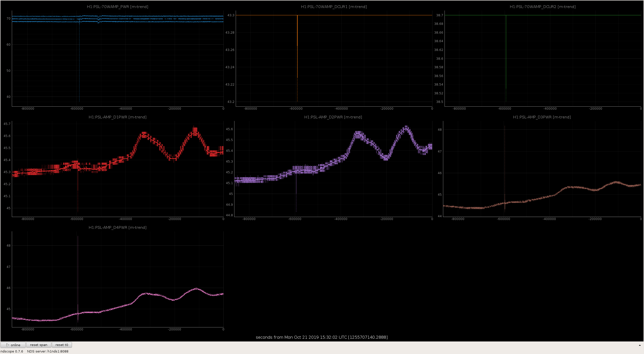
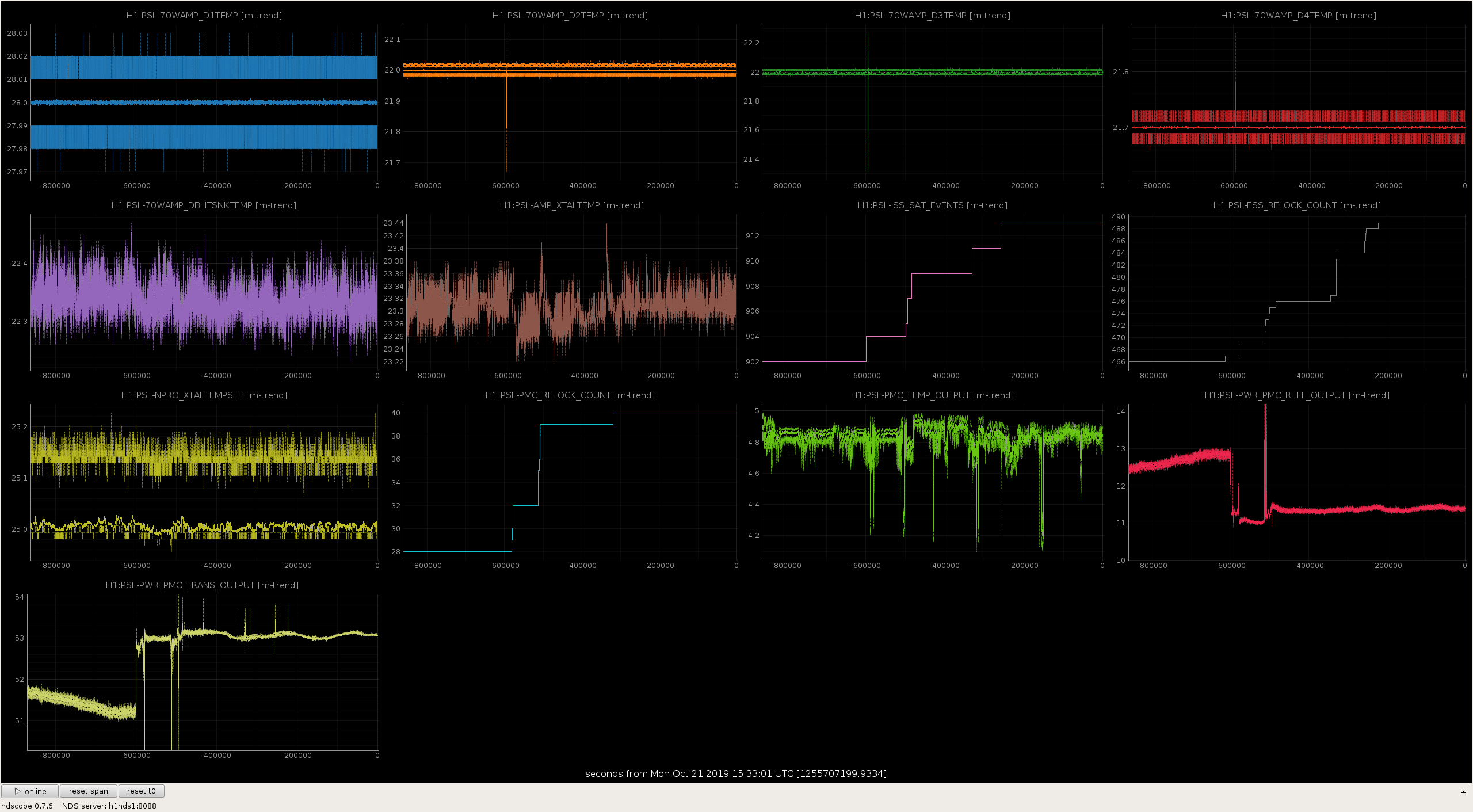
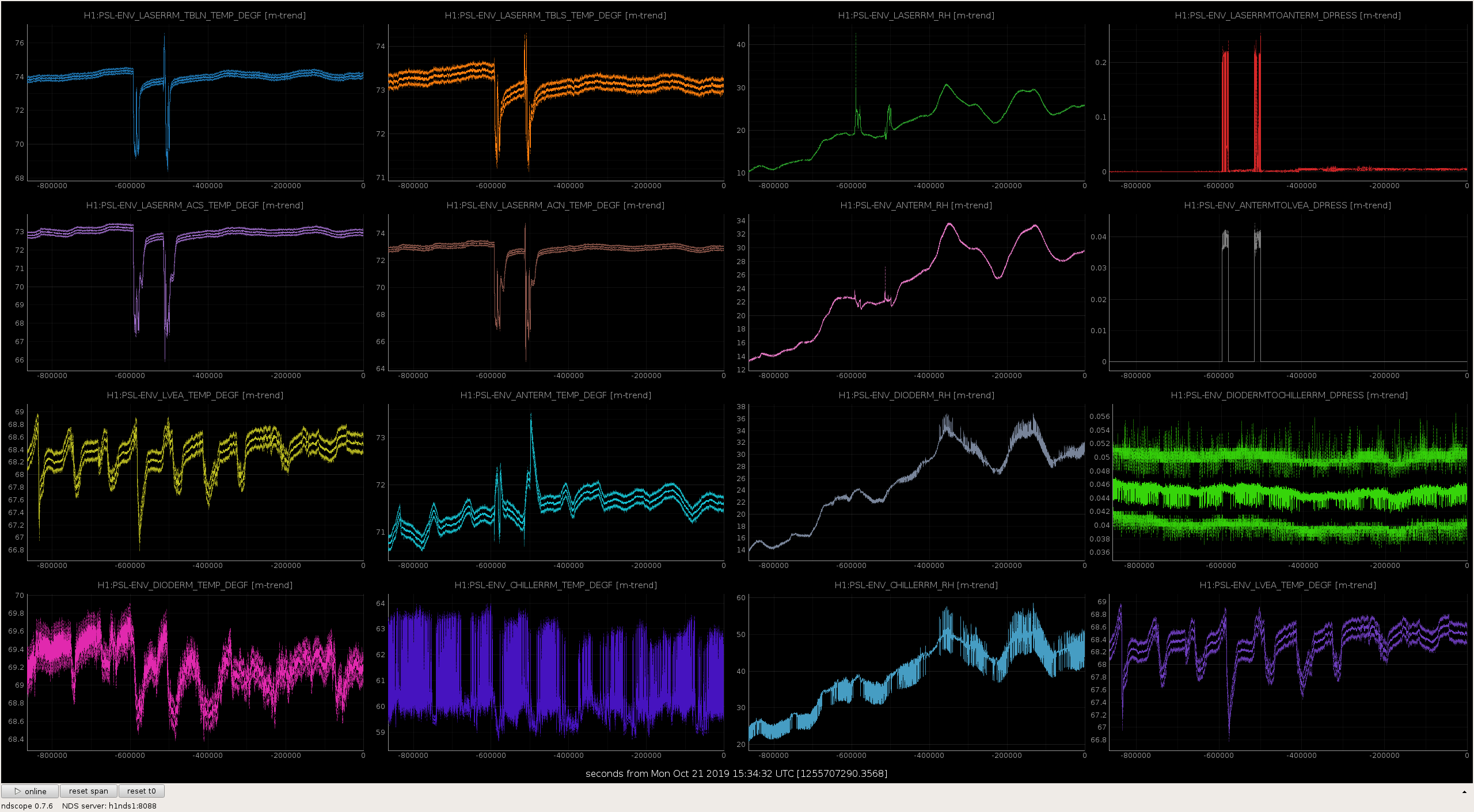
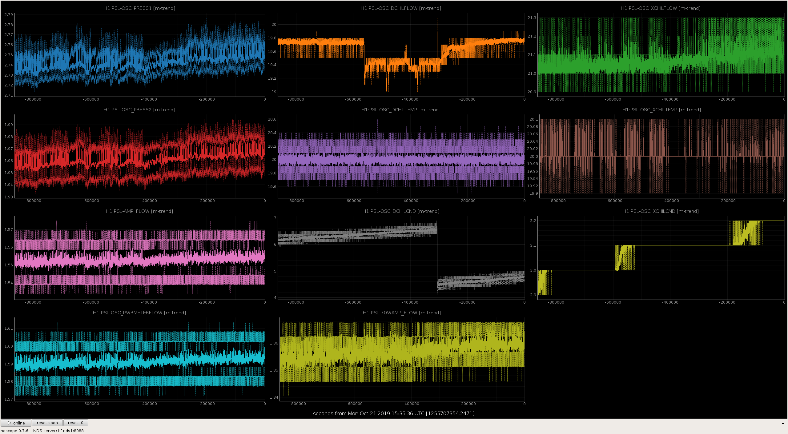
Varun, Stefan
We started writing an SRMI guardian state in the ALIGN_IFO guardian. It is not functional yet.
After aligning the DRMI (the input pointing was quite off), we started testing the SRMI state, but we ran into trouble with the fast shutter: It closed and we couldn't find out how to reopen it.
We lost instrument air pressure at the Corner Station for several hours today as others were replacing the compressor units. I had isolated the pneumatic pistons (closed 1/4 turn valves) for GV6 and GV8 prior to the loss of air pressure so as to minimize the stroking of the lead-screw belows but GV6 eventually sagged and the MEDM screens indicated a YELLOW status nonetheless. I reopened these isolation valves and fully stroked open GV6 and GV8 upon the return of air pressure following the compressor work.
Additionally, I had substituted bottled N2 in place of the instrument air line so as to maintain functionality of the electro-pneumatic isolation valve used on the HAM6 turbo backing cart so as to continue pumping HAM6 uninterrupted during the compressor replacements.
On Friday I leak tested the housing of the NEG pump, after some mixed signals I determined that there was no leak. The background on the leak detector remained around 4.5E10-10 torr*L/Sec.
Today I found out that one of the NEG controllers is misbehaving, it did not have the correct settings for the activation procedure nor the correct setting for a conditioning procedure, regardless of the pump or the procedure selected the settings remained the same. The NEG cable connection was moved to a different controller that had the correct settings. NEG pump 1 was activated without issues, and it's internal temperature reached the programed temperature of 550 oC. The gauge corresponding to this pump is currently reading at 2.31 x 10-07 torr.
The odd controller will be set aside and troubleshooted at a later time.
The NEG pump system will remain with the small turbo and leak detector attached until tomorrow, due to its internal temperature, last I checked the temperature inside the NEG was ramping down and the current temperature was 38 oC.
Jonathan, Dave:
As the first part of the upgrade of h1tw1 from its V1+RAID hardware (gentoo 2.6) to the all-in-one hardware (debian 8) (already done for h1tw0) I did the following:
During a 5 minute break time on both h1tw1 and h1tw3:
stopped daqd running on h1tw1, took this out of monit control, we are no longer running daqd on this unit
switched h1tw3 to write to a new minute_raw directory, its old data is now ready to be deleted since its disk is at 96% full
We then reconfigured h1nds1 (the default NDS server) to temporarily:
Serve recent archived data (24sep - 21oct) from h1tw1 while these data are being transferred to LDAS-GW
Serve current data (15:37 todays onwards) from h1tw3 using a temporary NFS mount point.
Because the raw minute trend 5-minute data blocks were not synchronized between h1tw1 and h1tw3, there is actually an overlap of a minute between the two data sets. It appears that dataviewer is insensitive to the data duplication, but ndscope gives an error (unexpected number of channels were received).
For a work around tonight, if you wish to use ndscope to get minute trend data, please use h1nds0 as your NDS server, for example
NDSSERVER=h1nds0:8088 ndscope -t yesterday -t now H1:PEM-EX_TEMP_ROOF_WEATHER_DEGC
we will work on the fix tomorrow.
Marc Daniel
We installed the new AOM driver for AOM1 in the CLF path. We measured 10.4dBm for the 200 MHz input (no attenuator needed). We adjusted the power gain of the driver to be at the maximum, but we have somewhat less RF power available compared to the old amplifier.
Some measurements at different drive points:
| Drive Point (V) | CLF launch (µW) | RF Readback (dBm) | Power meter (dBm) |
|---|---|---|---|
| 4.7 | 34 | 31.1 | 29.5 |
| 0 | 17 | 27.1 | 26.0 |
| 3.0 | 21 | 28.5 | |
| 10.0 | 47 | 33.4 | 31.4 |
The RF power meter was measuring at the table feedthrough. There is about 1dB loss in the cable from the AOM driver to the table. We chose 4.7V as the nominal for the drive point offset. The lower limit was set at 3.0V, and the upper limit at 10V.
The CLF launch power was 70µW before we switched to the new AOM driver. We have about ⅔ of the previous CLF power at the maximum drive point, and about ½ at the nominal settings. We could probably get most of the previous AOM diffraction power back by implementing an Isomet 505C-2 amplifier instead of the 505C-L, and by using a heliax cable. However, we have plenty of light available in the CLF path before the power adjustment stage, so this is probably not important.
TITLE: 10/21 Day Shift: 15:00-23:00 UTC (08:00-16:00 PST), all times posted in UTC
STATE of H1: Planned Engineering
INCOMING OPERATOR: Jeff
SHIFT SUMMARY:
Flurries of activities on site continue leading up to Gate-Valve opening later this week.
LOG:
Attached is a plot of the powers into and out of the green fiber, in the time since the pump down of HAM6.
The top panel shows the powers launched into the fiber, the rejected power (power in the wrong polarization which is rejected by a PBS right after the colimator on the OPO platform) and the power on the OPO reflection diode.
You can see that in the early part of the pump down the polarization rotated a bit. I adjusted the launched power to make some measurements of the nonlinear gain and threshold last week (52518), and after those measurements the OPO was on resonance for a while, which can be seen by the high OPO transmission in the second panel.
It seems that after I lowered the launch power and pulled the OPO off resonance, the transmission has increased a bit, to about 42% transmission of the entire chain, which is a bit better than we were measuring before the pump down. 52420
Note that the calibration of the rejected diode and the OPO reflection diode disagree, since we measured the calirbation of the REFL diode last week using a power meter, I rotated the polarization to maximize the rejected power then the reflected power, and muliptied the rejected power by 0.80 to correct for the difference.
Chiara, Jenne.
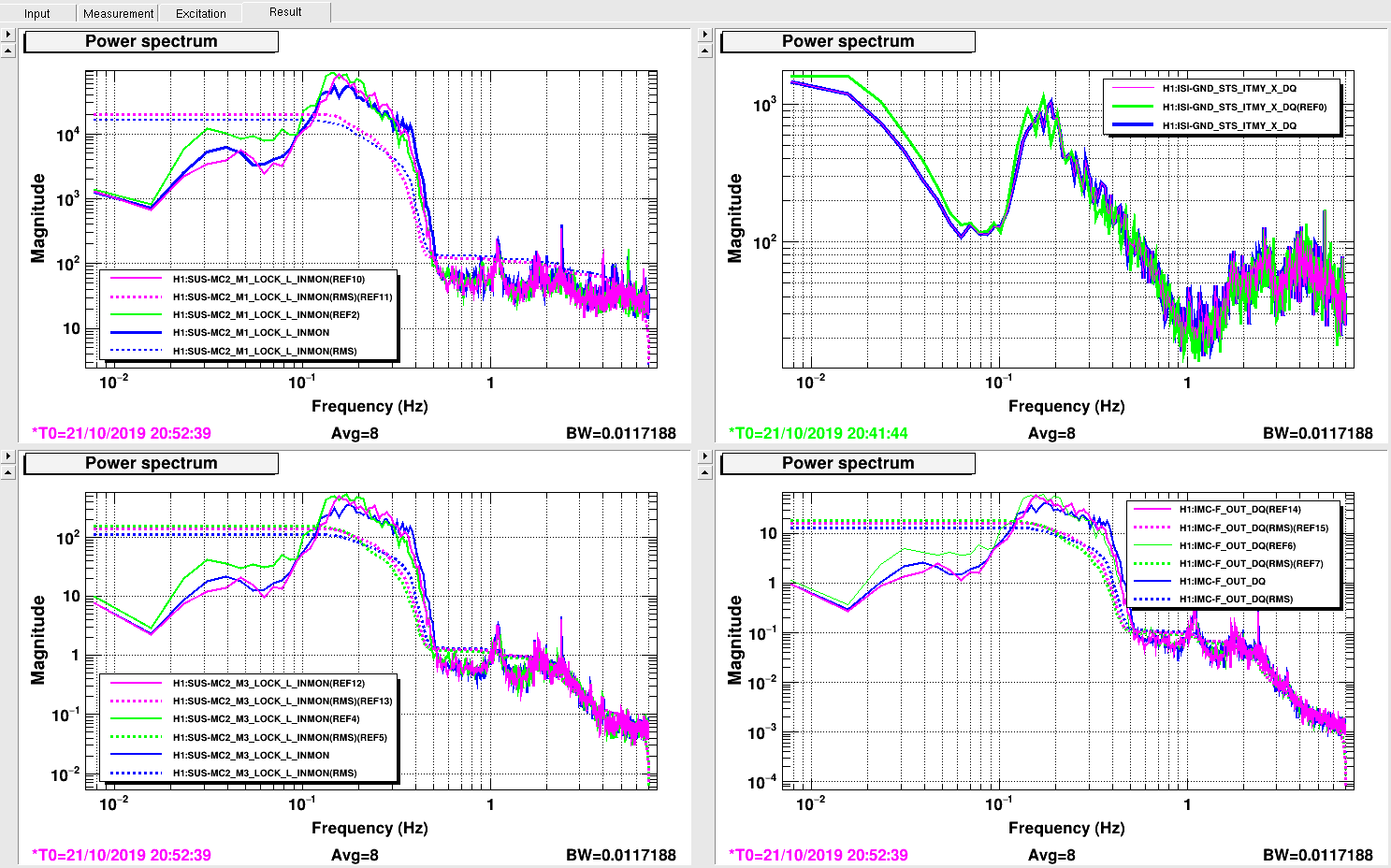
Today we tested the new configuration for ISI motion suppression through CPS feedback. We looked at the effect on MC2, ground motion and IMC; sensor correction was off everywhere.
First attachment shows the plots: we tested the system in OFF status (green trace) and in ON status, with two different 100mHz low pass filters, one called "100 mHz" and it is in blue trace, the other is called "new_lp" and it is in pink trace. Both filters are shown in the second attachment. We got a factor of about 3 of improvement at 60mHz.
With both filters there is an improvement below 0.1 Hz and the ground motion was always comparable. The new_lp filter already has an AC-coupling; next step will be to apply an AC-coupling also to the 100mHz filter and test again.
We left the system on. To turn it off, the gain on H1:ISI-HAM3_SUSINF_X has to be set to zero. To get here, open ISI -> HAM3 -> OFFLOAD screens.
PSL Report FAMIS report:
Laser Status:
Front End Power is 32.5W (should be around 30 W)
70W Output Power is 69.29W
Front End Watch is GREEN
70W Watch is GREEN
PMC:
It has been locked 3 days, 20 hr 52 minutes (should be days/weeks)
Reflected power = 11.37Watts
Transmitted power = 53.08Watts
PowerSum = 64.45Watts.
FSS:
It has been locked for 2 days 18 hr and 3 min (should be days/weeks)
TPD[V] = 5.138V (min 0.9V)
ISS:
The diffracted power is around 1.9%
Last saturation event was 3 days 3 hours and 35 minutes ago (should be days/weeks)
Possible Issues: None
Attached are the monthly trends.
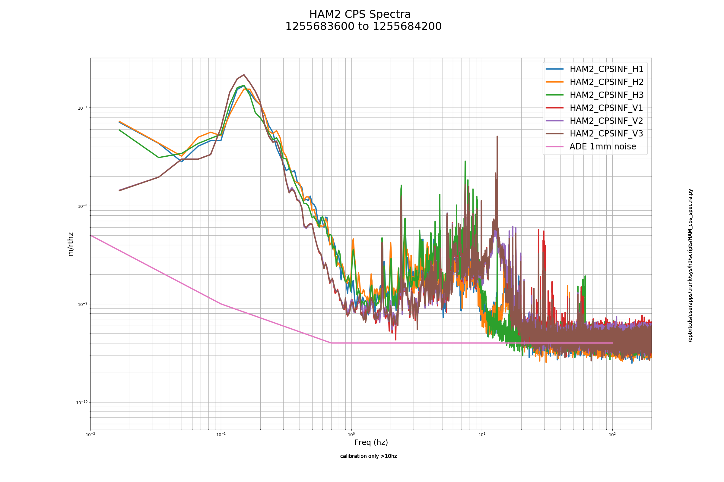
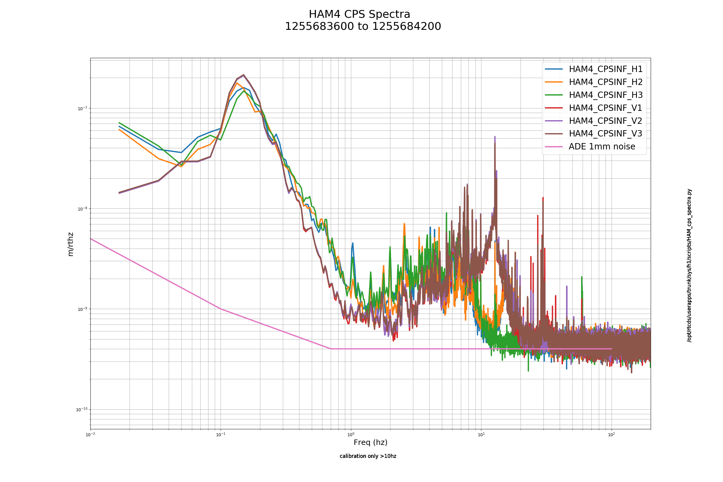
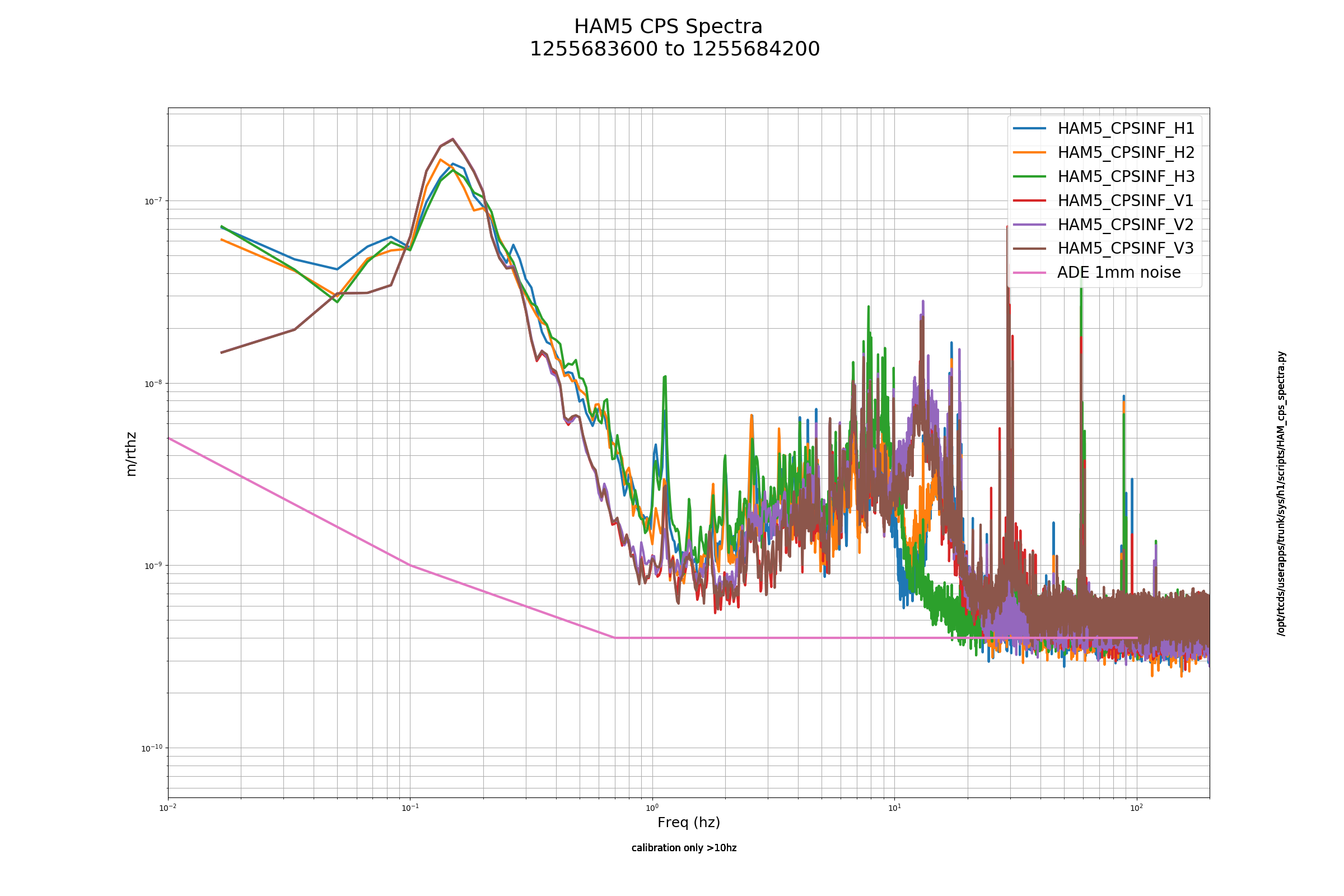
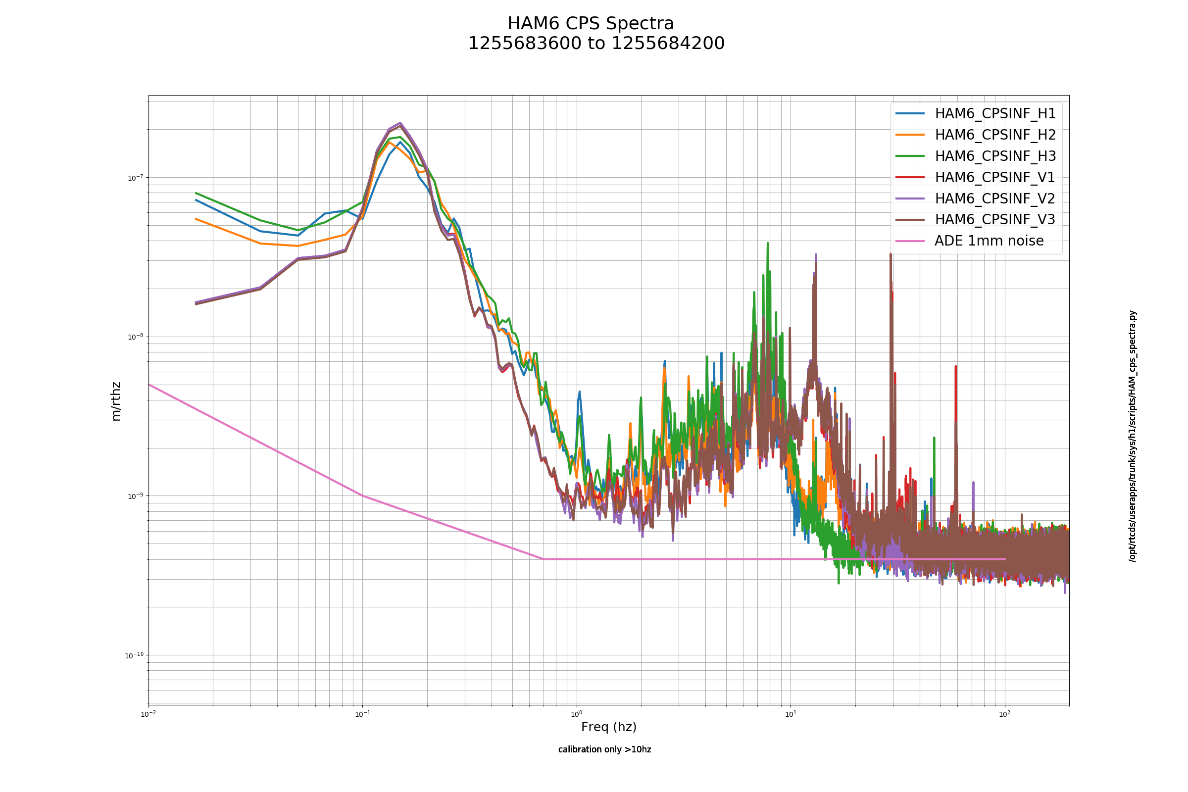
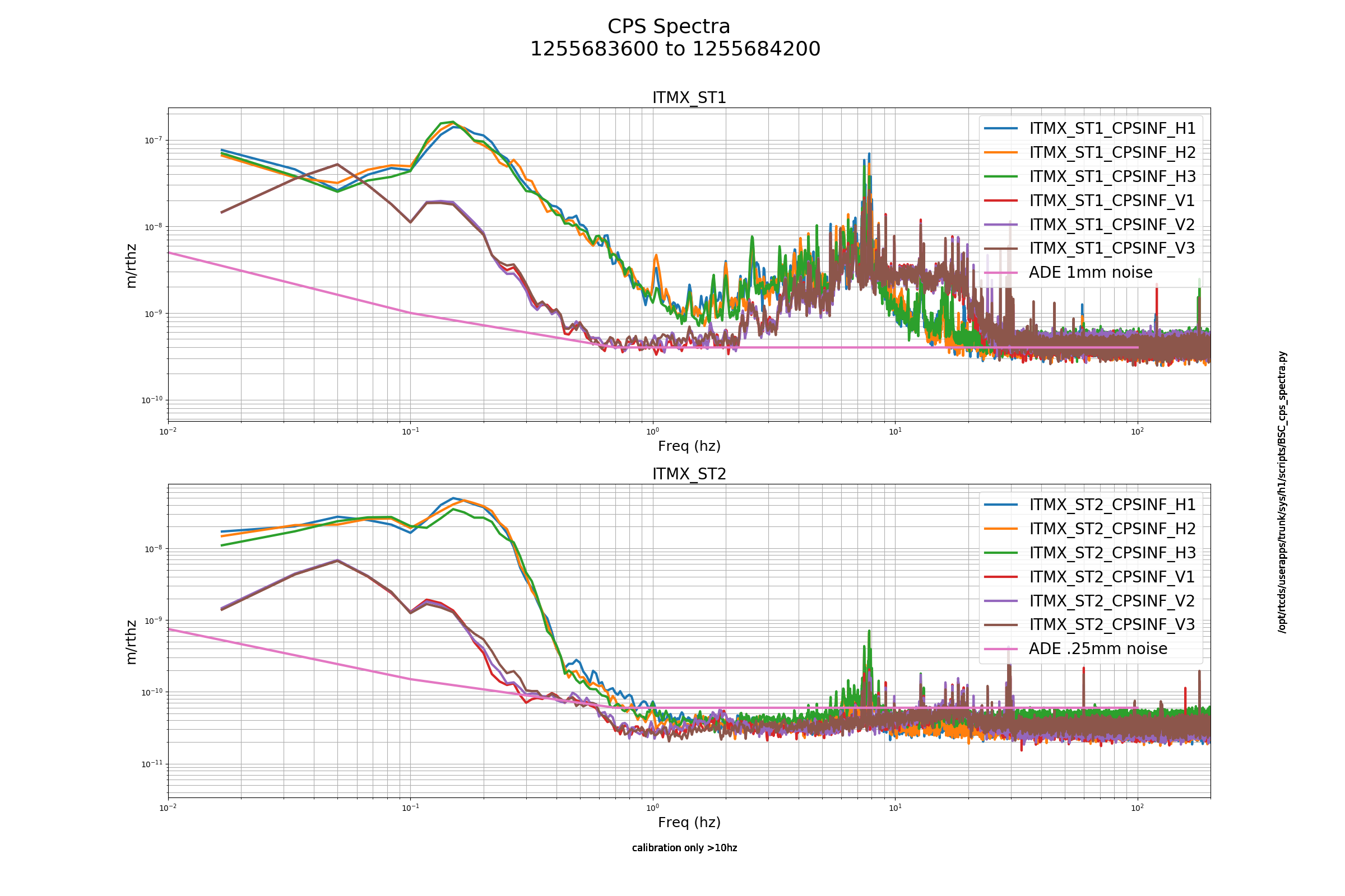
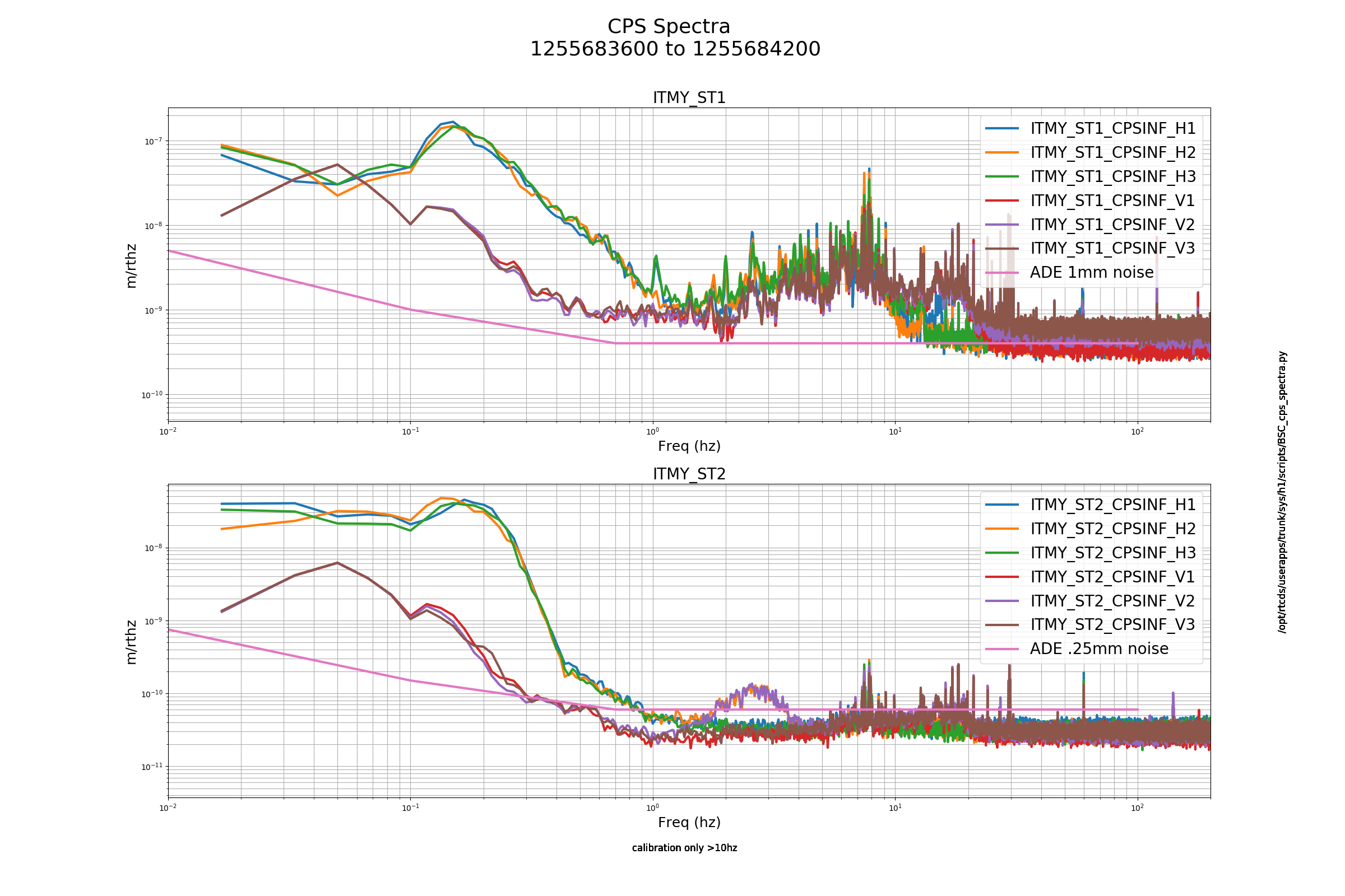
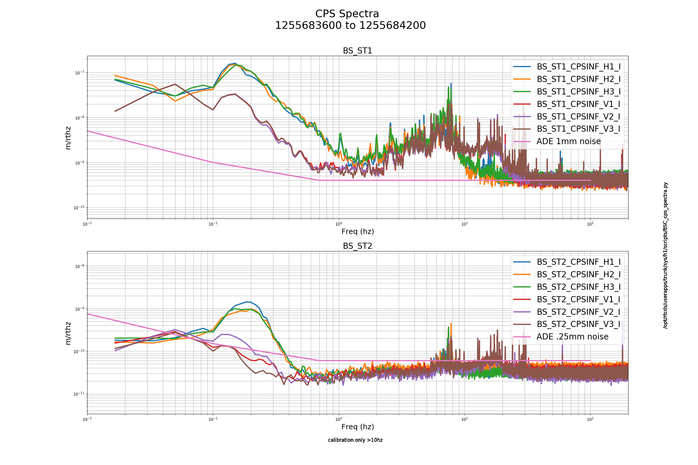
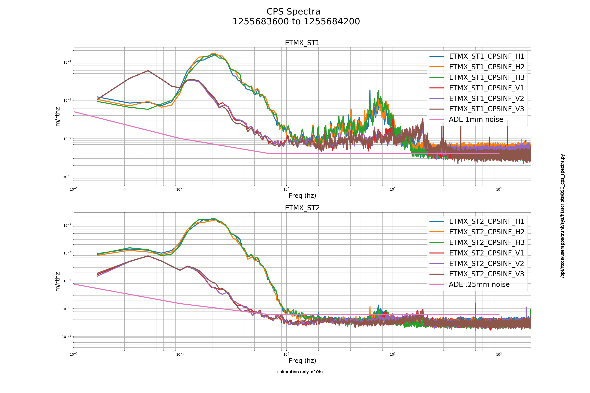
HAM & BSC CPS: All CPS' look good for high-freq range from attached plots.
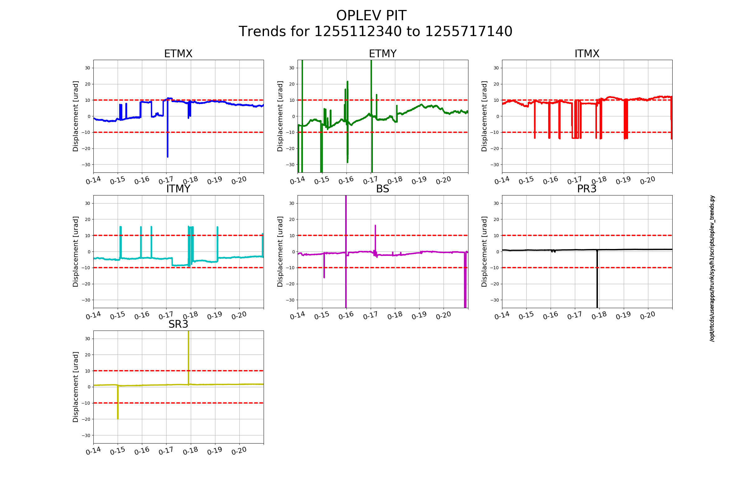
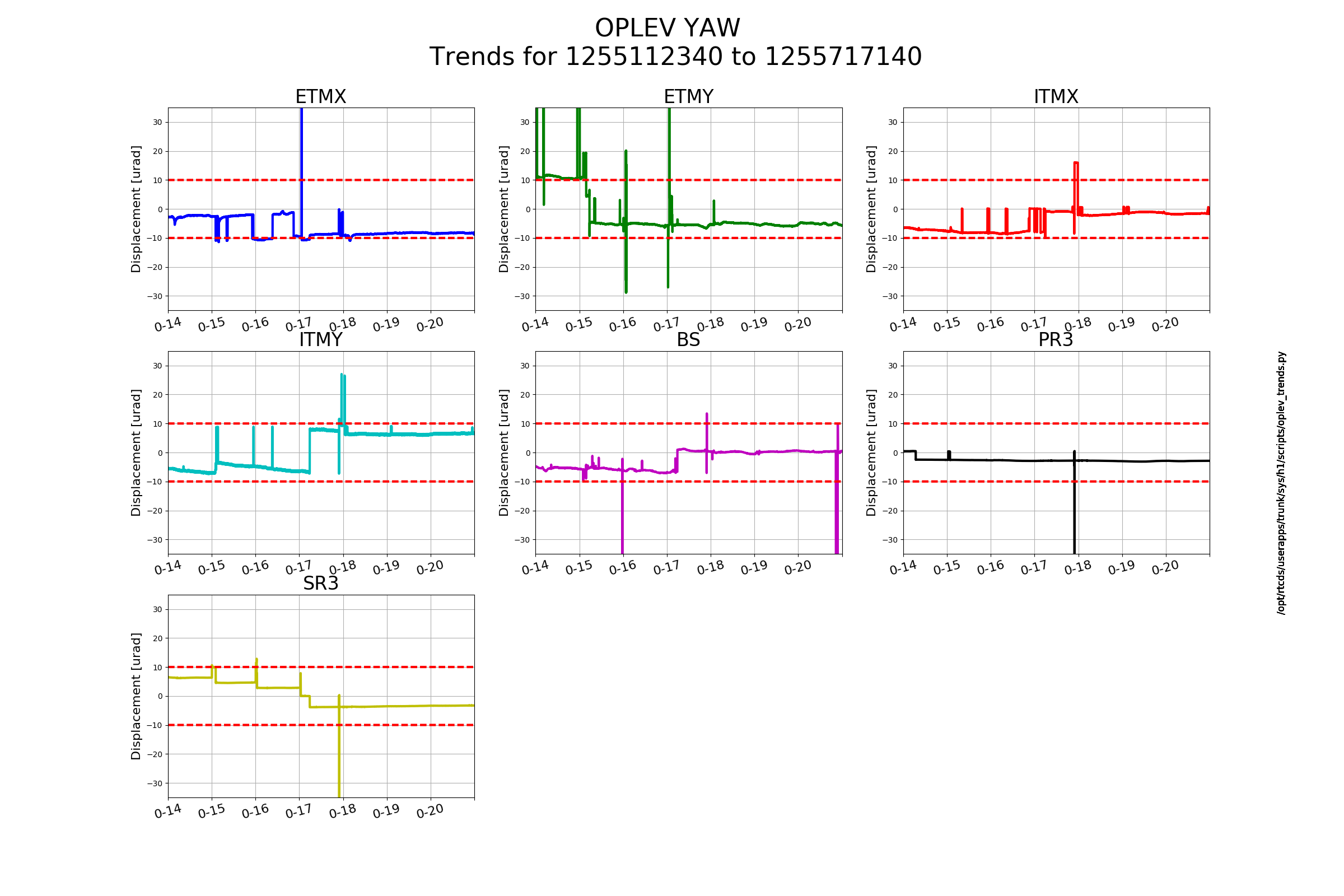
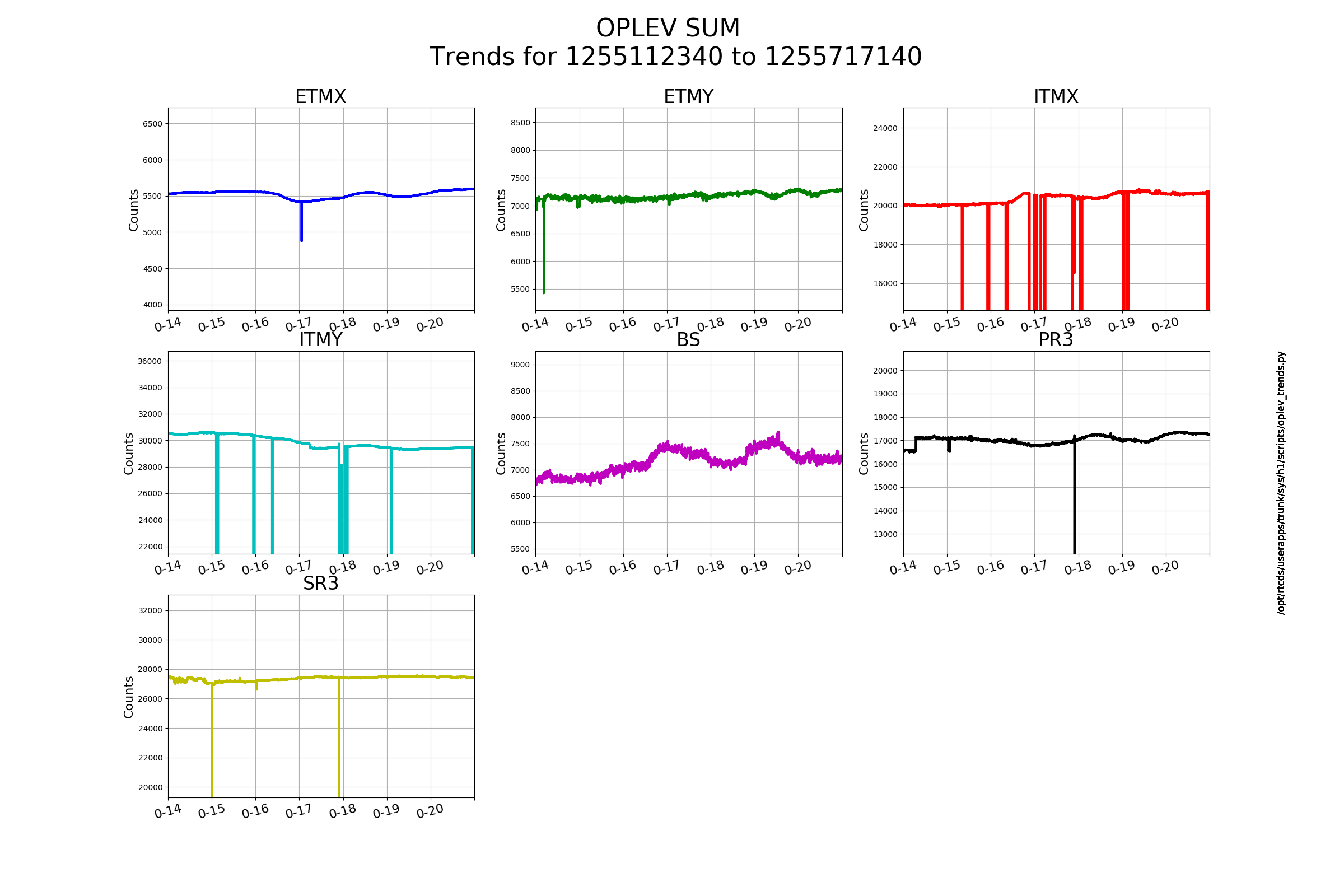
Attached are trends for oplevs.
NOTE:
This work is done as part of LIGO Ticket 12980:
https://services.ligo-la.caltech.edu/FRS/show_bug.cgi?id=12980
My goal was to propagate a transfer function in the form of zeros poles and gain (zpk) through python, into the filter banks generated by foton. There is a python version of foton, named foton.py, that wraps around the C++ libraries which foton is written in. This can be found on the gds SVN here:
https://redoubt.ligo-wa.caltech.edu/viewvc/gds/trunk/GUI/foton/
The end goal is to used this foton.py to import the suspension models (giant zpk arrays) directly through python.
This version doesn't support directly importing a zpk array, however Lee McCuller has done a lot of work upgrading this, and a beta foton.py can be obtained obtain from:
https://alog.ligo-la.caltech.edu/aLOG/index.php?callRep=38086
I tasked myself with testing this beta version, though getting it to run and run correctly took a lot of fiddling. This beta was written against a newer version of the ROOT library (which bridges the python code to the C++ libraries). There are a number of problems I ran into when trying to use the newer (not newest) version of ROOT on the control room computers, which I can summarise in saying that it needs to be installed and configured properly to run anything. My solution (for testing purposes) was to strip sections of code that relied on new functions of ROOT which did not exist in the version currently used on those systems. At some point I needed the libssl.1.0.x library to run some part of ROOT - this is not installed on the control room computers, so I downloaded the library and copied locally to a folder so ROOT can use it if it is needed.
My working beta version in question is posted here as [fotontst.py]. I did find a tiny bug in Lee's code that breaks the ZPK functionality: [line 527 in foton.py from Lee's code] should be "zero_list.append(matlab_complex_str(zero))", so that zero's get pushed to foton.
Steps for testing [all in python 2.7]:
1) [test_foton/zpk_create.py]. I wrote a short script to create a matlab-like .mat array file, that contains zeros,poles and gains of some filter. I compared against the data structured imported from the susmodel arrays to make sure it is the same format. I used a 6th order elliptical filter to create a nice shap feature as the reference. This output is [testdata.mat].
2) [test_foton/zpk_foton.py] through [test_foton/run.sh]. [run.sh] imports the libssl library (from the lib folder), runs the [zpk_foton.py] script, and copies the new filters file to the directory above it. [zpk_foton.py] simply reads the .mat file, passes the data into the ZPK_set functionality of the beta version of [fotontst.py] into a specific filter block that was unsused, and writes it out. Final file is [H1CALCS_from_py.txt]
3) [H1CALCS_from_foton.txt]. I use fotons gui interface to create a filter (ellip("LowPass",6,1,40,35)) with the same parameters and save it to this file. [diff.txt] is the difference between [H1CALCS_from_py.txt] and [H1CALCS_from_foton.txt]. You can see the small numerical differences you might expect would arise from slightly different number precisions used in C++ and Python to generate the transfer functions.
4) [tf_compare/foton_tf] and [tf_compare/foton_tf]. These two files are outputs from within foton's gui. I output the transfer functions as an array of frequency, real, imaginary. This is done for the filter generated through foton [foton_tf] and filter generated through python and imported in steps (1) and (2).
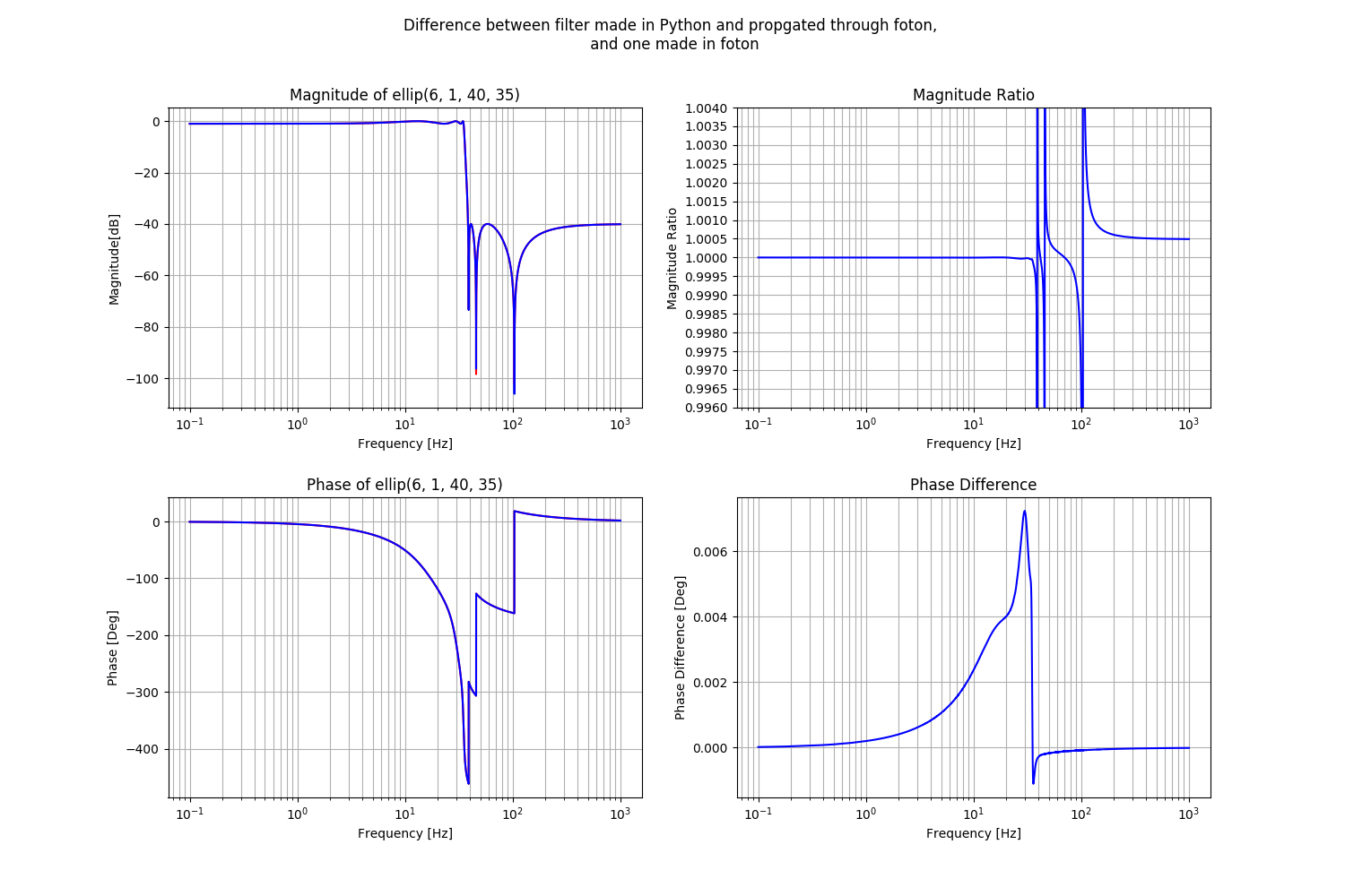
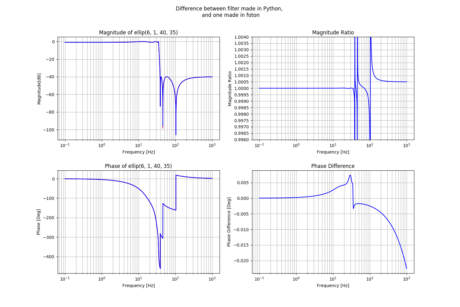
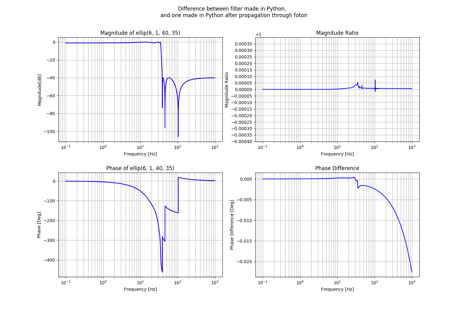
5) [tf_compare/tfcompare.py]. This script compares transfer functions and spits out pretty pictures like [pyth_vs_foton.png], [pyth_vs_pyth_through_foton.png] and [pyth_through_foton_vs_foton.png]. I tested the tree combinations of comparisons for:
a) [pyth_vs_pyth_through_foton.png] make the filter in python and compare it against the same filter after it has propagated through the foton in steps (1) and (2).
b) [pyth_vs_foton.png] make the filter in python and compare it directly against the filter made in foton.
c) [pyth_through_foton_vs_foton.png] python filter after it has propagated through the foton compared against the filter made in foton.
Result discussion:
5a) [pyth_vs_pyth_through_foton.png]. This is the important one. This compares the same function propagating through foton and comparing it against that it was originally in python. As you can see there is minuscule changes in the magnitude ration on the order of 0.005%, which is probably numerical error on fotons output. This is the key plot, since the goal is to check if importing a ZPK array though foton.py and comparing that against what you started with should be the same. Notable also, is the phase difference at high frequencies, as this points to some difference in how TFs of ZPKs are handled between foton and python.
5b) [pyth_vs_foton.png]. Here we compare a filter directly made in python vs the output from foton. We see a similar phase error as the case above, and we see spikes in the magnitude ration arising from small numerical differences in the positions of the poles and zeros. What is relevant is the 0.05% difference in the magnitude ratio at high frequencies, but that differences (as I have been told by Jeff Kissel) is acceptable.
5c) [pyth_through_foton_vs_foton.png]. This one shows that the phase difference vanish when you are looking at data outputted from foton - indicating that the phase difference at high frequency in 5a and 5b isnt really real, and is a difference to how python vs foton calculate the phase from ZPKs at the output. The magnitude error is the same as 5b.
Conclusion:
The goal is to take a 'known good' array of ZPK data and propagate that to a filter bank. Remember that in importing the susmodel the ZPK arrays are already made so there is no extra numerial error to add there. The magnitude error from 5a is relevant here as that checks reproducibility. 5a sees some phase offsets that are not seen when both data sets are outputted from foton (5c), pointing to a difference there which would not be seen when importing susmodels.
All in all, it looks like foton.py is importing the filters correctly with minial error, and should be fit to import data from a complete susmodel. Next step is to produce a plot similar to 5a that looks at how python plots the TF based on the ZPKs vs how foton plots the ZPKs of the huge susmodel array.
The bypass on HAM6 vacuum (PT110) has expired, this gauge is now below its alarm level of 5.0e-06Torr.
While work is ongoing with the corner station compressed air supply, I have bypassed this channel for a few hours.
Bypass will expire:
Mon Oct 21 16:50:28 PDT 2019
For channel(s):
H0:VAC-MR_INSTAIR_PT199_PRESS_PSIG
SAFETY:
Coordination Activities:
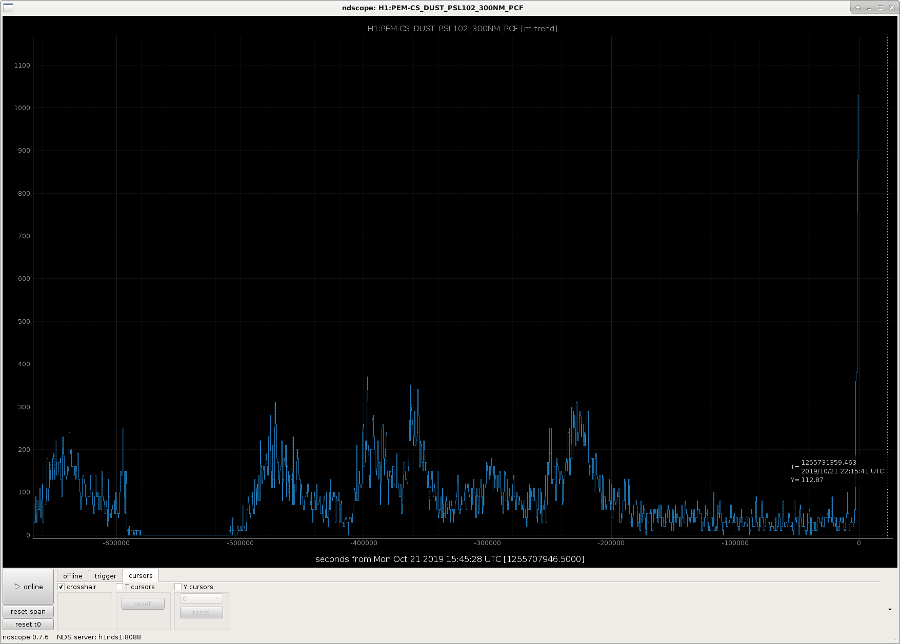
At 8:35 a PSL Dust Monitor went into a MAJOR dust alarm state for 0.3um particles. It generally stays around 0-300 counts, but at 8:35 it jumped up to 1000+ counts (see attached screen shot). Will notify Jason/Jeff B.
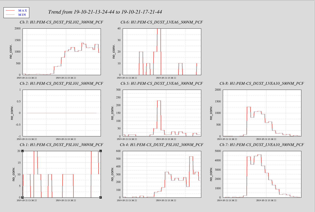
Klye was wet drilling in the west bay this morning between ~14:30 (07:30) and 15:15 (08:50).
Starting at 14:38 (07:38) the particle counts in the Bier Garten (LVEA10) spike up and drop back to normal by 17:00 (10:00).
Similar behavior is observed in HAM6 dust monitor (LVEA6). It starts to climb 14:48 (07:58) and drops off by 15:22 (08:22) - The HAM6 counts are elevated but only to 230 0.3um and 40 0.5um particles.
The dust monitor (PSL101) in the PSL Enclosure did not any counts for the 0.5um particles and no more than 20 of the 0.3um particles.
The Ante-Room-Room dust monitor (PSL102) spikes at 15:00 (08:00) however Ante-Room does not clear out like the rest of the monitored spaces in the LVEA. At the last check (17:50 (10:50)) the counts were 750 0.3um particles (alarm limit is 700 counts) and the 0.5 um counts are in the 200s.
See attached plot.
The PSL Ante-Room air is supplied by any overpressure from the LVEA and enters through vents in the bottom of the enclosure. The exhaust fans are not running during these times. Therefore there was no HEPA fan extraction of air from the Ante-Room and no corresponding air exchange. This is why the counts remained high in the PSL Ante-Room. Given the current design of the PSL Enclosure, if there are particles in the LVEA room air and the exhaust fans are on in the PSL Ante-Room these particles are going to be drawn into the PSL Anti-Room.
The 0.3um counts are still above the minor alarm level but getting better.
Keita, Dripta, Georgia
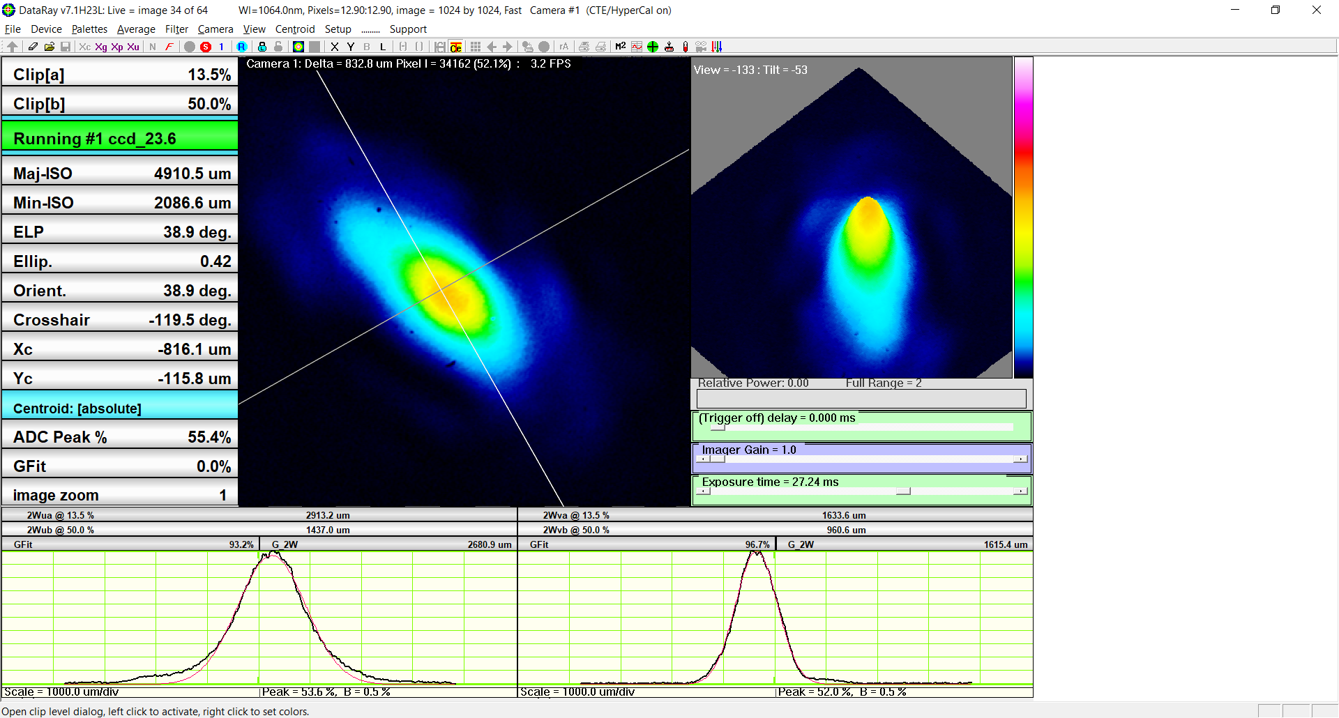
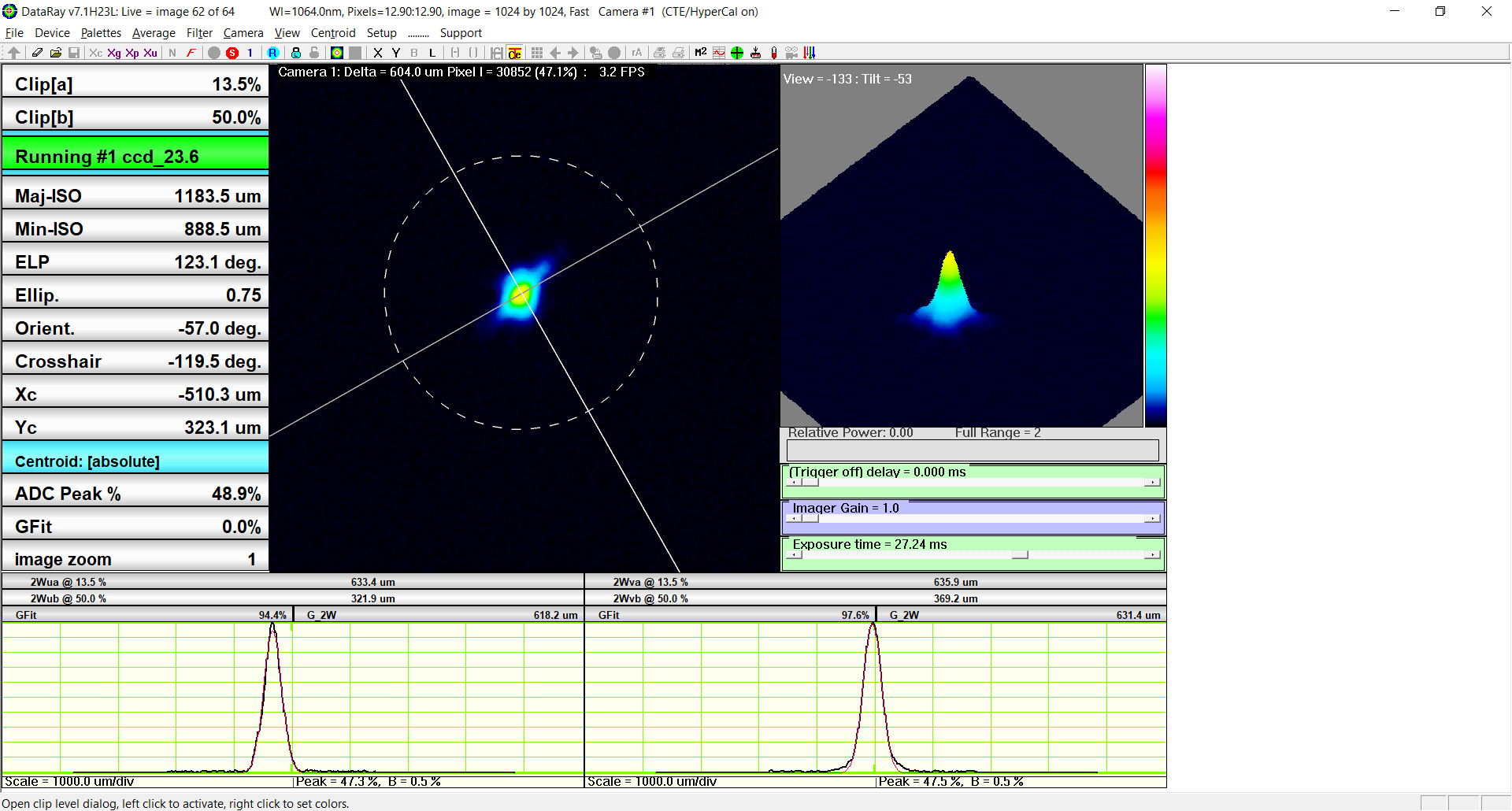
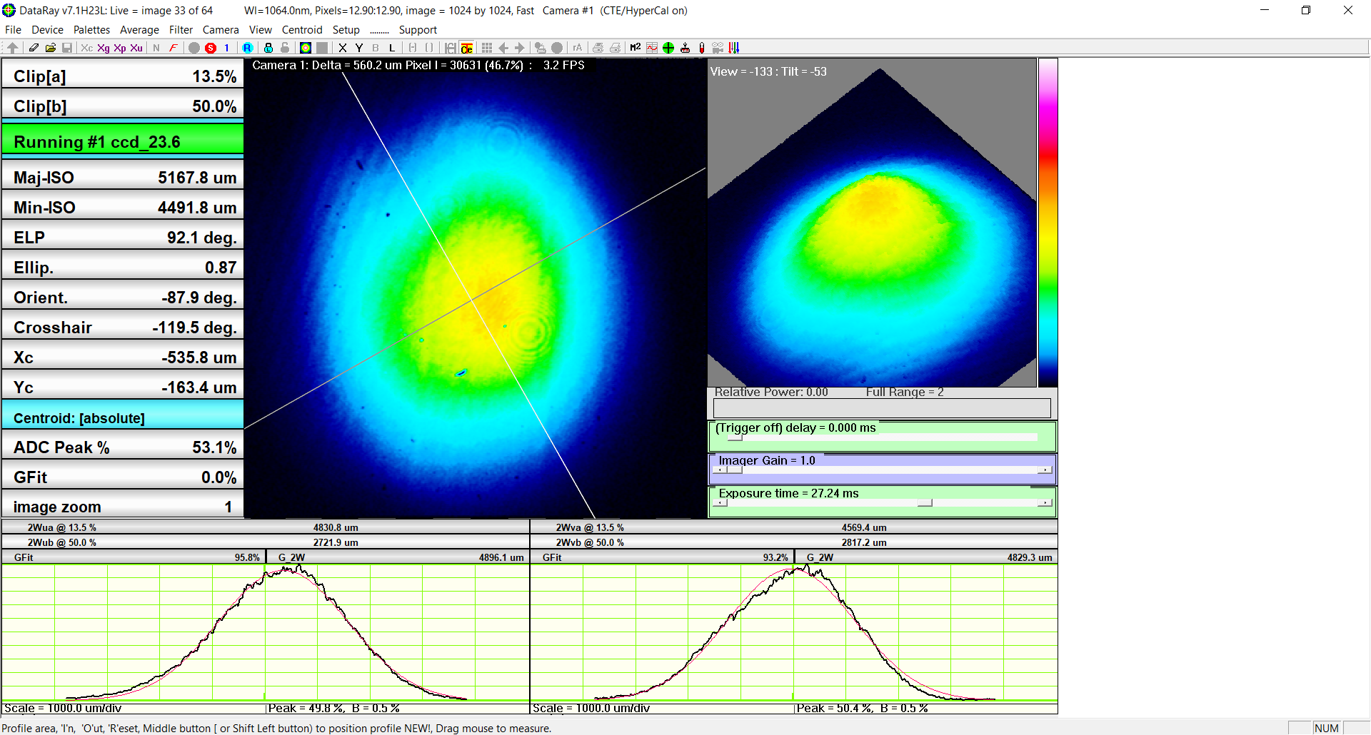
Today we continued investigating the poor mode matching of the ALS-Y green beam, following on from work eariler in the year. We took some new photos and used the wincam camera profiler to look at the beam. We haven't solved the problem but we noted that:
Next week we might monitor the profile of the reflected beam while adding offsets to the QPD servo, which will change the beam position on the transmon optics, to see if there is some clipping.
1. Viewport beam spot position
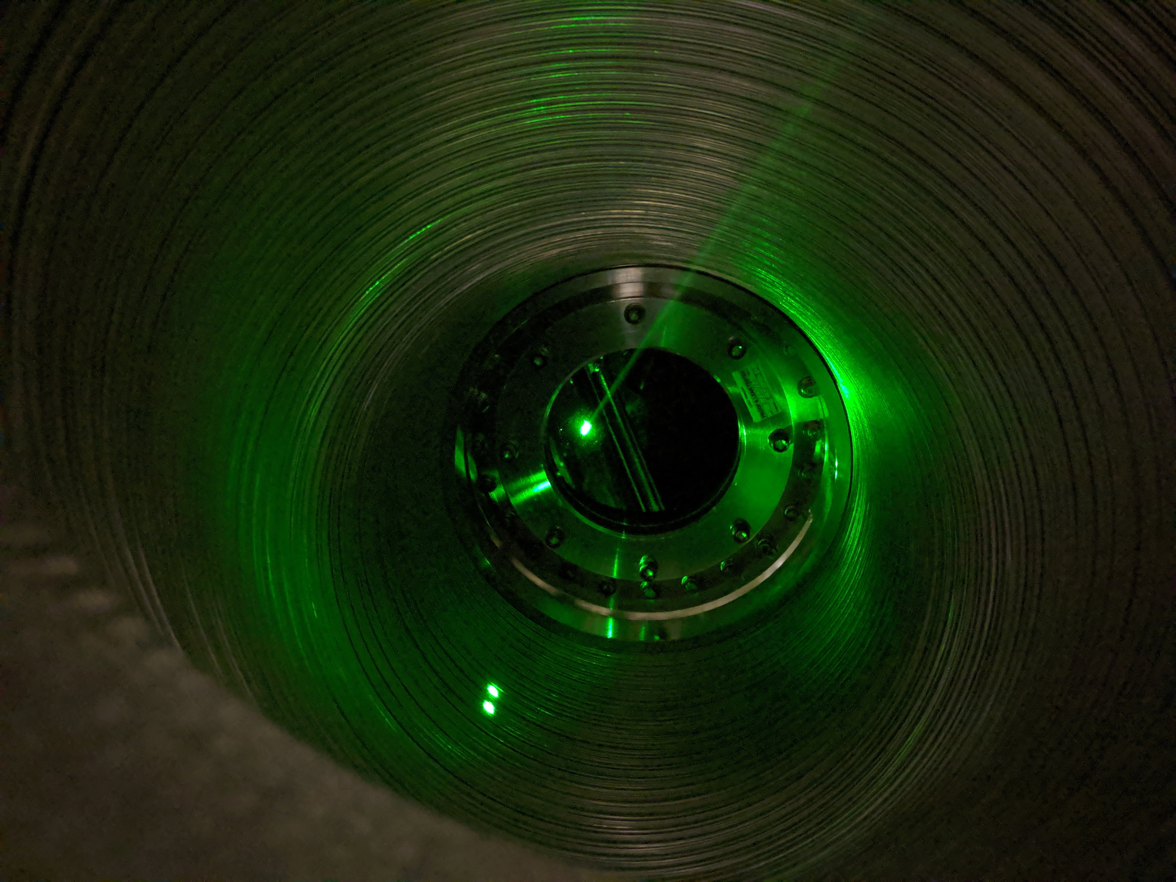
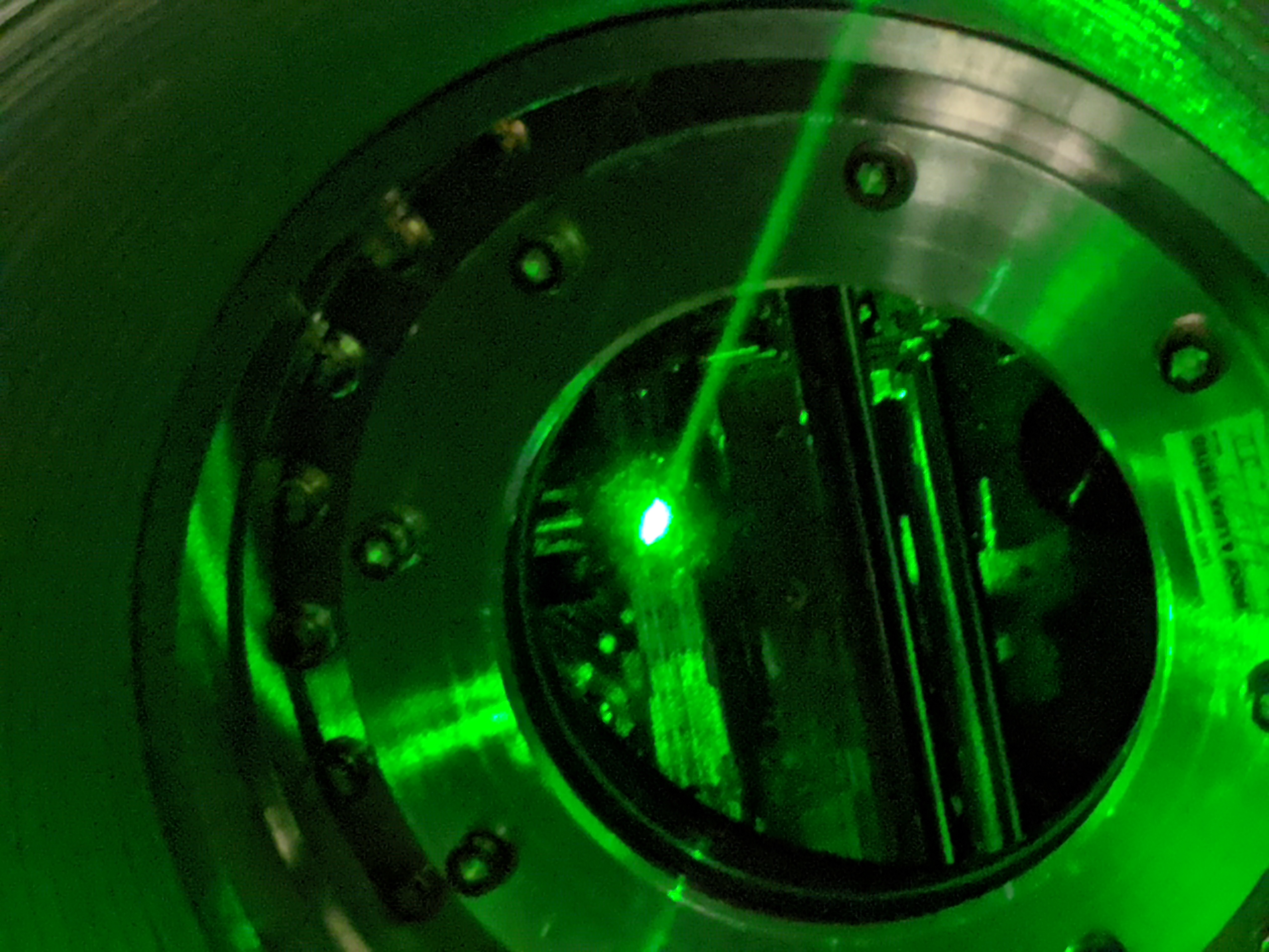
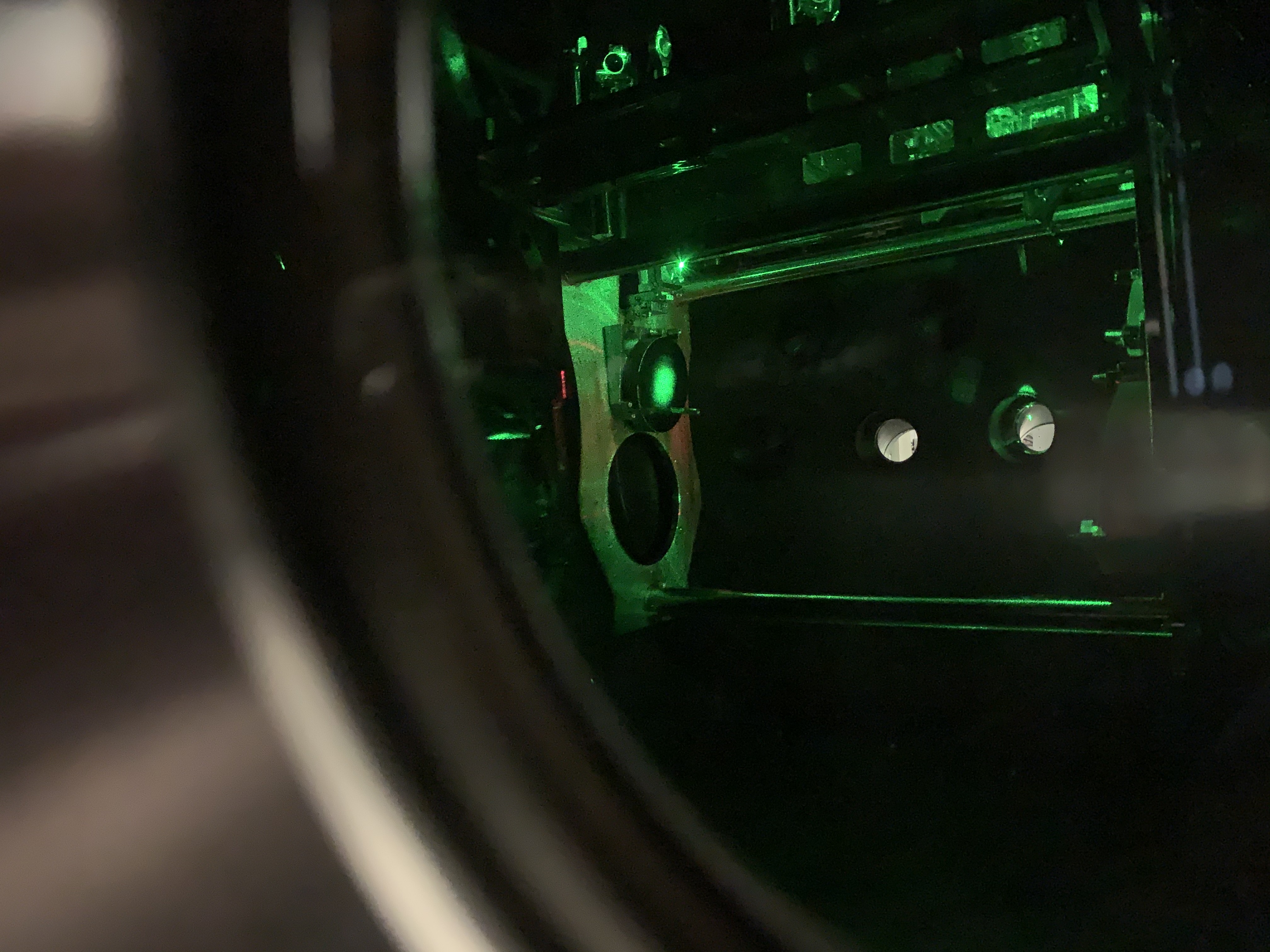
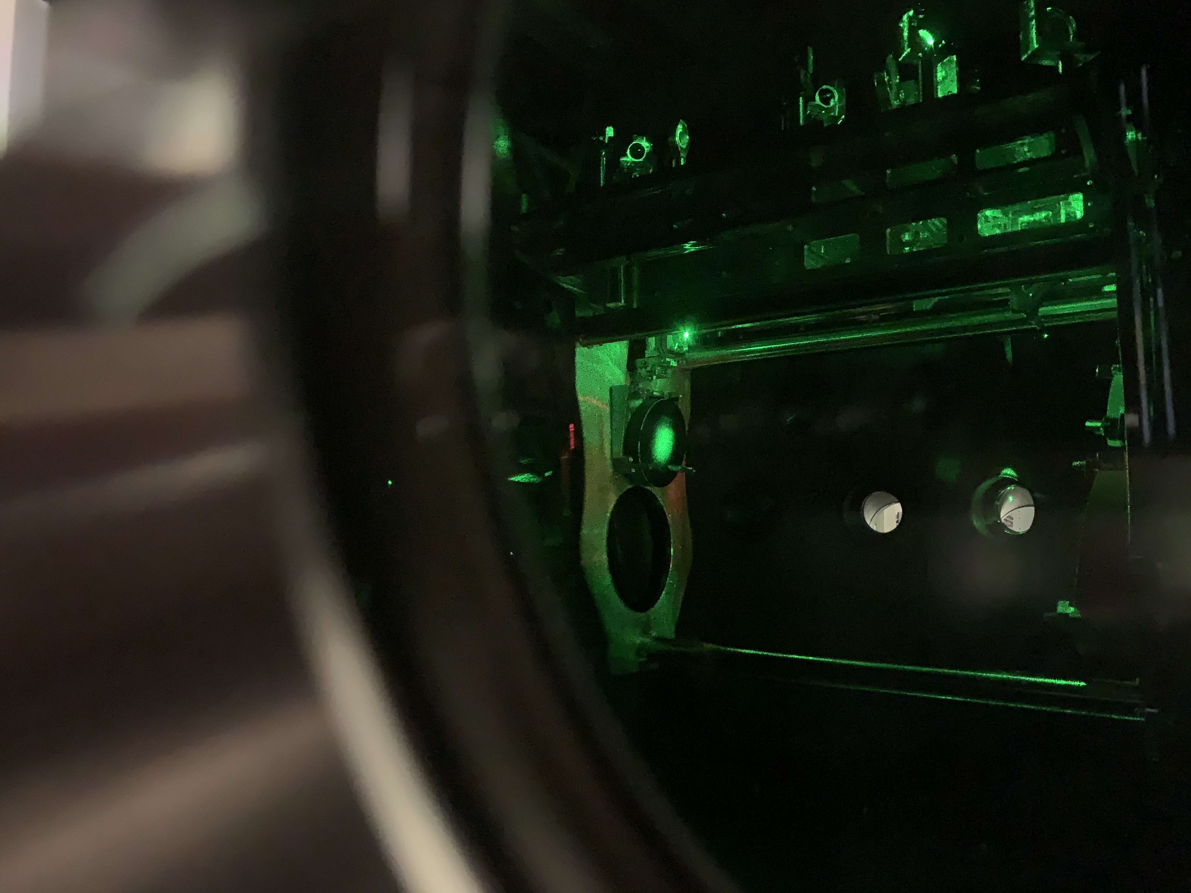
1st and 2nd picture show the beam position on the viewport. In the first picture you can also see the two AR ghost beams hitting the inside of the duct material.
That the beam is close to the edge of the viewport will NOT affect the polarization but could affect the beam shape as the edge of the viewport is not really flat and could act as an irregular lens. We don't know how much the effect is at the current beam position, though.
(In the past, Pcal team found that excessive amount of aberration observed in ITM pictures taken with large aperture telescope (see e.g. the last page of https://alog.ligo-wa.caltech.edu/aLOG/uploads/35327_20170404172516_IrLowPower_reduced.pdf for example) is not observed in their tests outside of the vacuum chamber, and that it is mitigated/eliminated by simply limiting the input aperture of the telescope, which means that the viewport surface is not flat at the edge.)
2. In-chamber TMS optics spot position
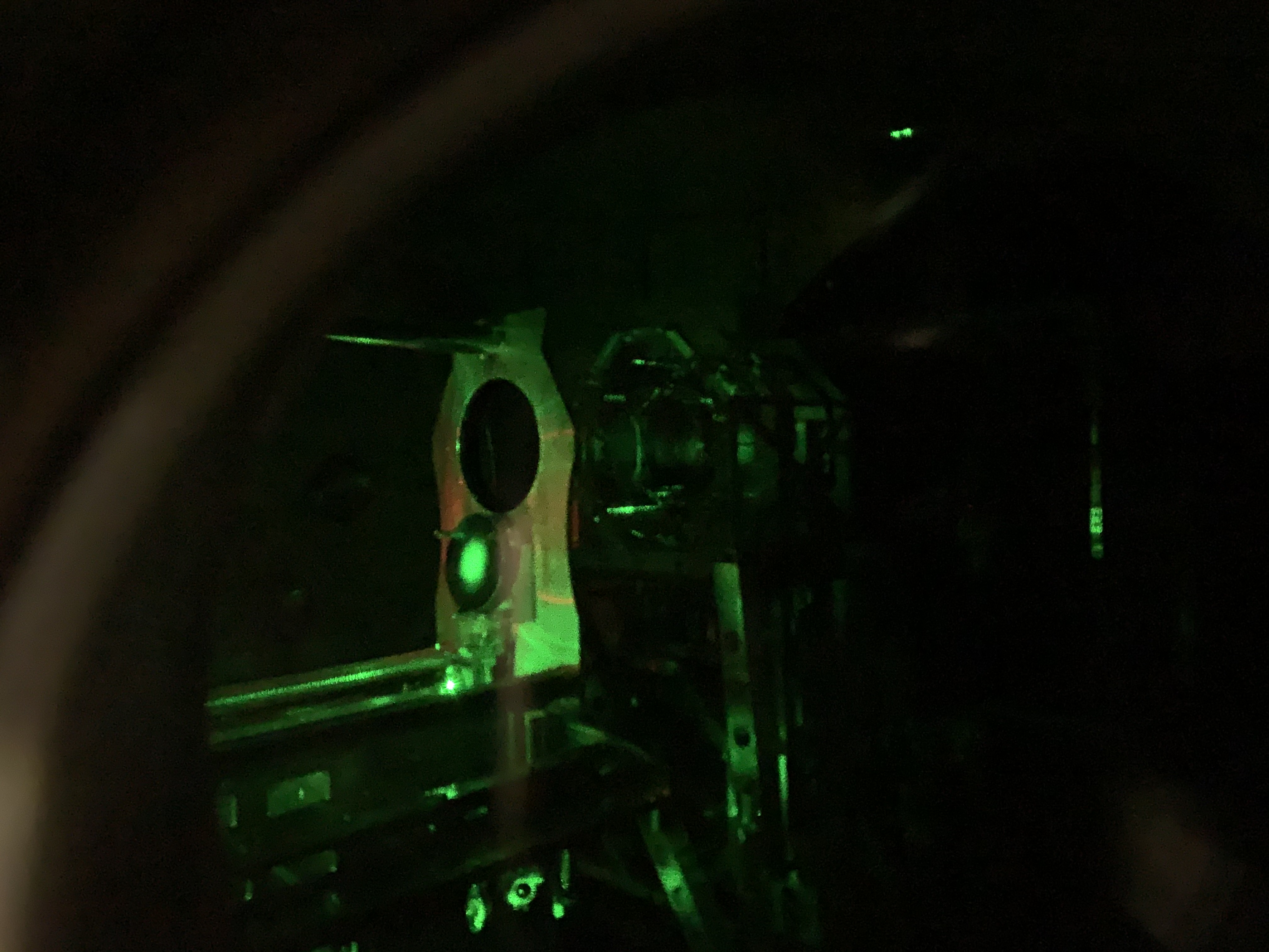
See this one VID_20191018_170216.mp4 on G1902047 showing the primary (big mirror at the bottom) and a flat mirror above the primary. Centering on flat mirrors doesn't matter that much. Anyway, it may be a bit low on the primary but I don't call this bad.
3. Green Polarization
It's only a minor problem for capturing the beam shape of the return beam (and a minor problem for ALS in general), and the first picture of Georgia's entry is entirely valid, but it might be somewhat interesting to think about the cause of wrong polarization.
When we placed a HWP upstream of ALS-M11 in D1400241 to minimize the transmission of the incoming beam on ALS-M11 (i.e. wrong polarization), the brightness of the return beam (i.e. coming back from the chamber) transmitted through ALS-M11 was still much brighter than that of the wrong-polarization incoming beam (and it didn't change much when we rotated the HWP because ALS-M11 is a PBS and we're not changing the polarization of the beam going into the chamber, just the power).
That the return beam in wrong polarization is brighter than the input beam in the wrong pol cannot be explained by geometric rotation of the polarization axes alone. If it's just geometric rotation, what is sent in comes back with the exact same polarization because ETM is retroreflecting and the return beam exactly follows the incoming path, cancelling the rotation effect.
It could however be explained by a combination of geometric rotation and polarization-dependent optics in chamber. For example dichroic mirrors are spec'ed for green S but not P (see e.g. E1000669). Green BSs seem to be spec'ed for P and S (e.g. E1000870), but no test data is supplied for P. Even though the ALS periscope on the ISCTEY (and ISCTEX) is designed to elliminate the geometric rotation such that S pol on ICST stays S pol on TMS, it cannot be perfect.
Attached are the pictures Dripta took of the transmon viewed from the camera viewport. There is a lot of scattered green light.
From alog 51458 we know that the 00 mode is only about 70% of the total power.
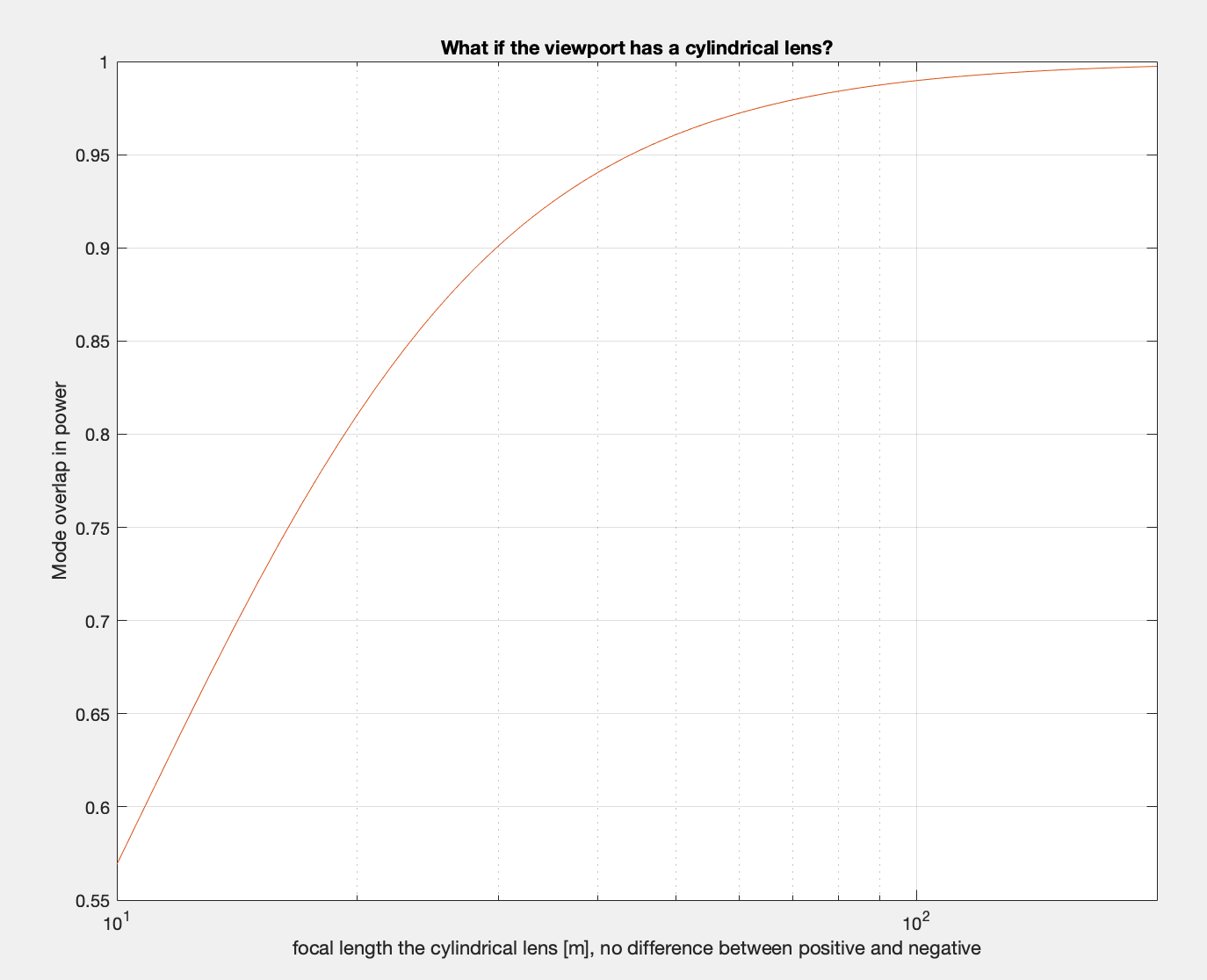
If we want to explain this using some kind of weird lensing on ISCTEY of on the viewport, the lensing needs to be large. Just to have some understanding of how large, here's a calculation of the effect of the elliptic lensing of the viewport.
I assumed that the lens is cylindrical so the mode shape is only altered in one direction, and plotted the mode overlap of the lensed beam and an ideal beam in power, not amplitude, as a function of the lens focal length.
To degrade the power coupling to 70% just by using a cylindrical lens, you need the focal length of about 14 meters. That's a huge effect, unlikely to come from high quality viewport D1101006/E1100267 as the transmission wavefront error is specified to be within lambda/10 for 633nm over the clear aperture of 5.2".