{Gerardo, Tyler, Kyle, Chandra, in various phases and combinations}
Core drilled the three remaining anchor locations at x-beam manifold turbo station and installed the threaded inserts. The existing turbo frame was cut via band saw to make clearance for Hilti equipment. Custom mods to one or two anchor brackets are required for this station due to core drill clearance issues.
Jeff. K, Niko, Rahul
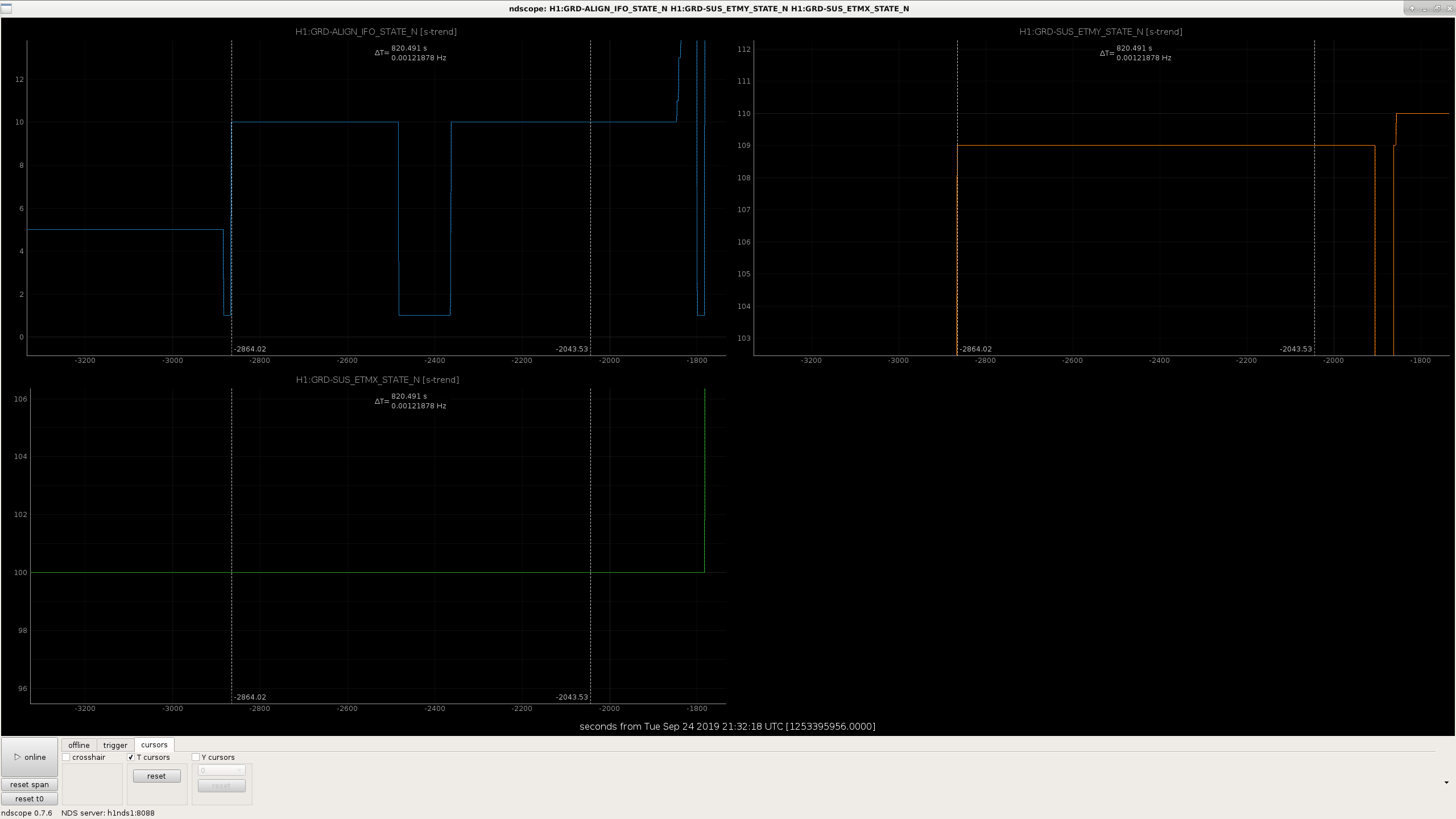
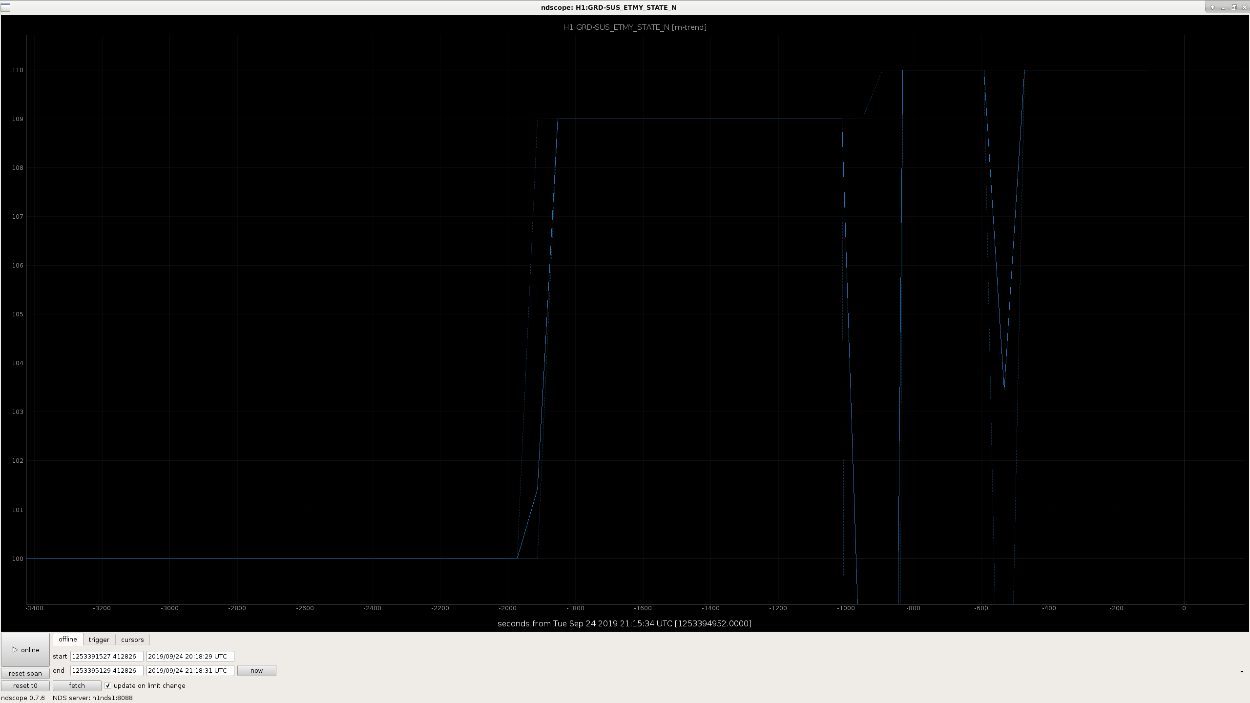
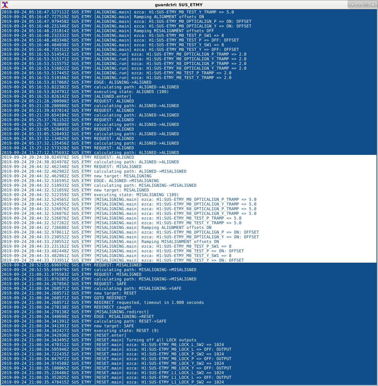
After the scheduled Tuesday maintenance, during IFO lock acquisition attempt, we found that the ETMY Guardian got stalled and got into MISALIGNING STATE (as per NIKO, ETMY also tripped this morning). In order to understand, what's going on, we looked at the channel H1:GRD-SUS_ETMY_STATE_N along with the log file (screenshots attached). Initially, Guardian was at ALIGNED (100) state and while attempting (with several requests) to jump (via 109 state) to MISALIGNED state (110), it got stuck at MISALIGNING (109) state. This can be seen in the highlighted section of the log file. During this time the Align IFO (H1:GRD-ALIGN_IFO_STATE_N) went from SET_SUS_FOR_ALS_FPMI (5) to DOWN (0) state and then to PREP_XARM_IR (10). Finally, Guardian went into SAFE and then RESET state.
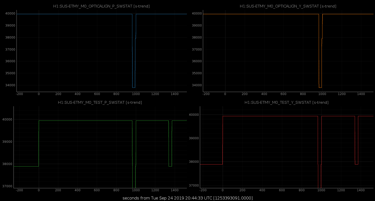
This seems to be another case of FRS13563. The SUS alignment filters' ramp values gets stuck on, and the check in the run method of the MISALIGNING Guardian state was waiting for them to clear. In this case, it was the TEST banks that seemed to have gotten stuck. The wierd part is that the SWSTAT value of 39936 is True for the gain ramping, not the offset like the node just changed (pythonic check: bool(39936 & 1<<12) => True).
I've only noticed this with the SUS banks, but they just use the LIGOFilter object that the rest of the Guardians use.
Tagged CDS, FRS, and GRD. Removed AOS tag.
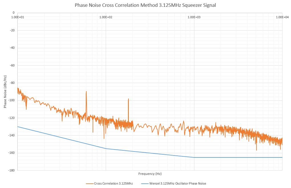
Due to the Engineering F2F last week, the cross correlation phase noise meauserment was rescheduled for this week. We measured the phase noise on the 3.125Mhz source located in the CER using the BluePhase 1000 Phase Noise Test System along with Rich Abbott's excellent notes on this measurement to hopefully nail this phase noise. The first attempt is located in this ALOG 51551.
First step is to measure the mixer slope which I found to be 44.2mV out of the IFR at 100Hz bandwidth.
Second step is to lock the frequency sources to the signal under test and measure the UGF of the system at 100Hz bandwidth which I found to be 34Hz.
Next we measure the PSD using FFT cross correlation.
Finally we adjust the raw FFT with the transform based on the first two steps as follows:
Loop Factor Compensation = ABS((20*LOG10(SQRT(1+(UGF/F)^2))))dB
Mixer Slope = 20LOG10(Vpp/(0.02*PI()))dB
Preamp Gain = 60dB
SSB Correction Factor = 3dB
Transform = FFT + Loop Factor Compensation - Mixer Slope - Preamp Gain - SSB Correction
I have attached the plot which is using a locking bandwidth of of 100Hz. After playing with the numbers I have found 10kHz locking bandwidth would give us an answer closer to the expected values from the notes.
Here is the link to the 3.125MHz Oscillator for reference:
https://dcc.ligo.org/DocDB/0140/T1700016/001/Wenzel_500_30576.pdf
Here is the link to Rich Abbott's application note for this measurement:
https://dcc.ligo.org/DocDB/0161/T1900434/003/iLigoVcoPhaseNoiseAnalysis_v3.pdf
While trying to scan the higher order modes in the OPO the green trans camera wouldn't show any beam. The camera turned out to be misaigned. This was fixed with a short incursion into SQZT6.
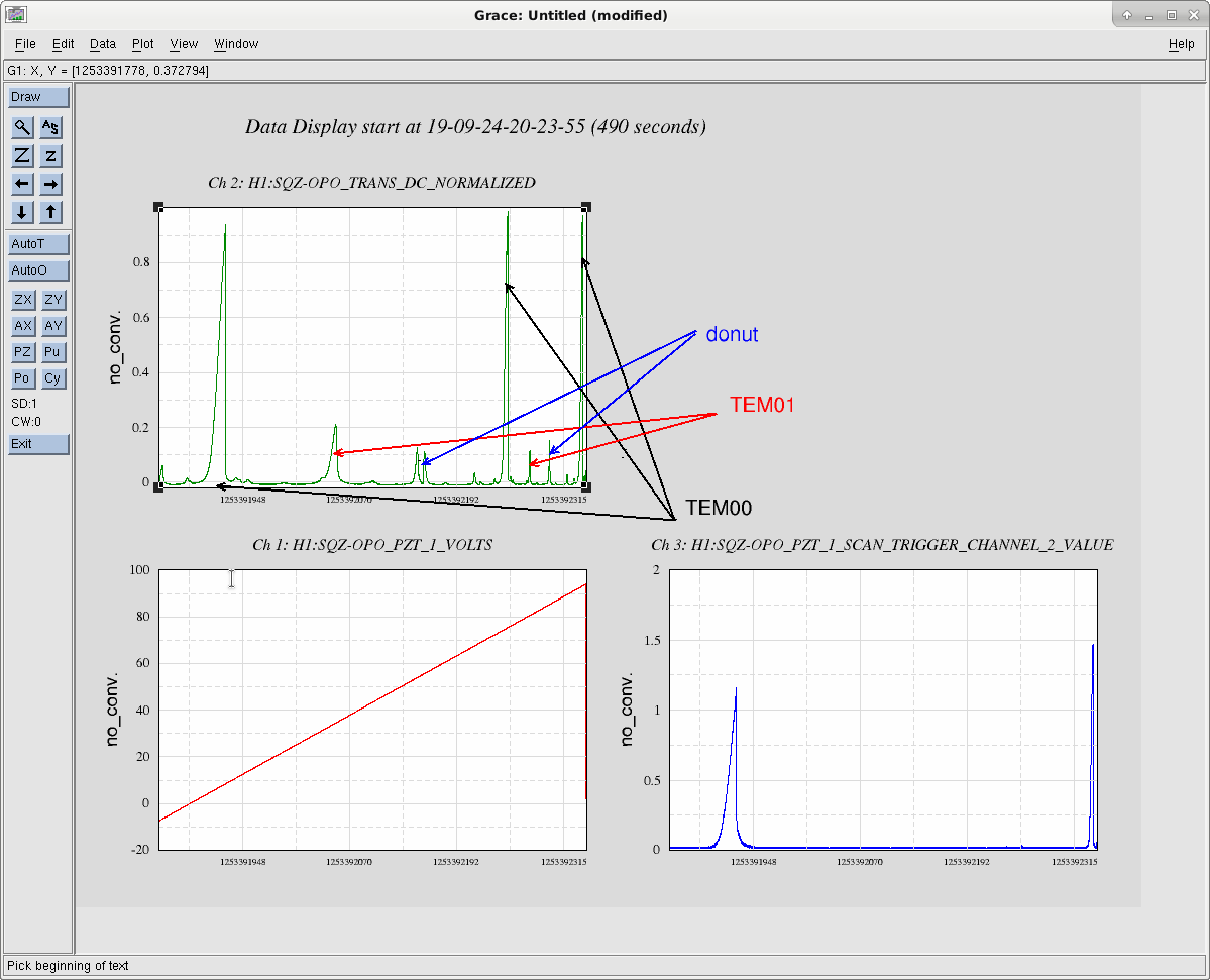
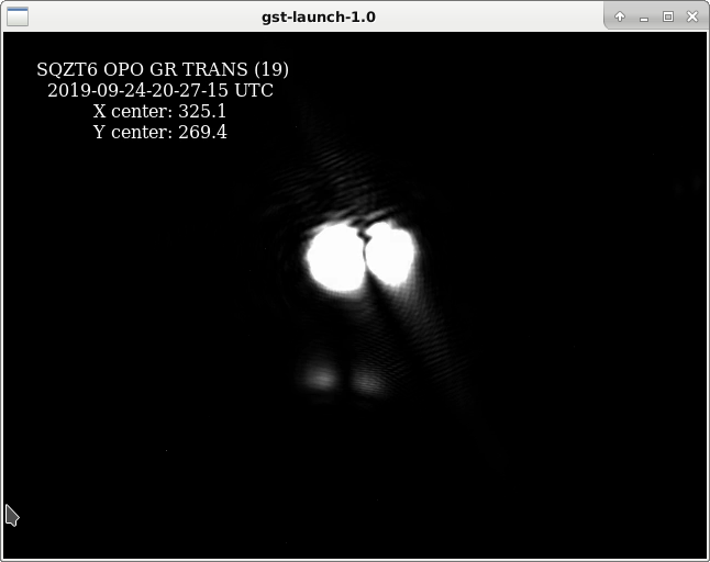
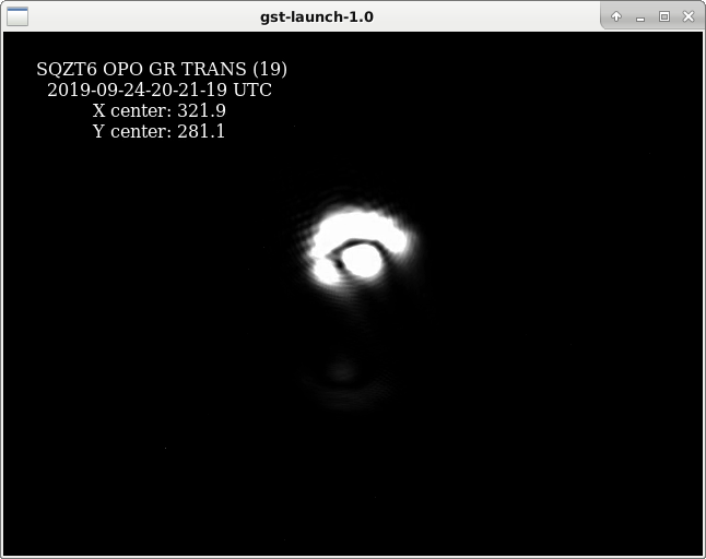
The plot below shows a typical scan. The next 3 snapshots show a TEM00, TEM01 and donut mode resonances, respectively.
The donut mode always seems to have an amplitude around 12-14% of the carrier, whereas the TEM01 mode seems to be larger at lower PZT values. The highest I observed was 25% (near 0V at the PZT) and the lowest around 10% (near 100V PZT offset). In the center of the range the TEM01 seems to be around 15%-20%.
I tried to verify this by locking at different carrier PZT offsets. With 23.3mW at the fiber launch point, when locked at -7V offset the transmitted power was at 89%, When locked at 49V or 92V, the transmitted power was both at 96%. So, at the very low end we seem to loose about 7% in the build-up power. Even so the trend is the same as with the scan results, it doesn't agree very well numerically.
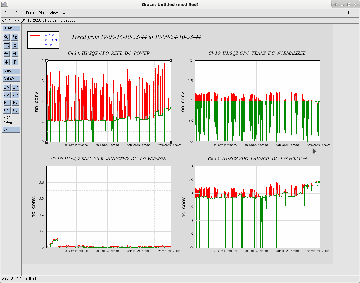
Lookig at the trends in the last plot, we can see that the launch power as well as the OPO reflected green power has started to increase around mid August, while the transmitted power was kept constant. The reflected power has increased by about 50%, whereas the launch power increased by about 25%. This looks like the fiber has started to degrade again.
I check the actual volatge put out by the PZT driver. If you ask for 100V it will output 100V. However, the readback is about 5% short of this. Looking at the schematics, the monitor is a resistive divider 240K/12K that is directly fed to a Beckhoff terminal. From experience the later has about 250K input resistance.
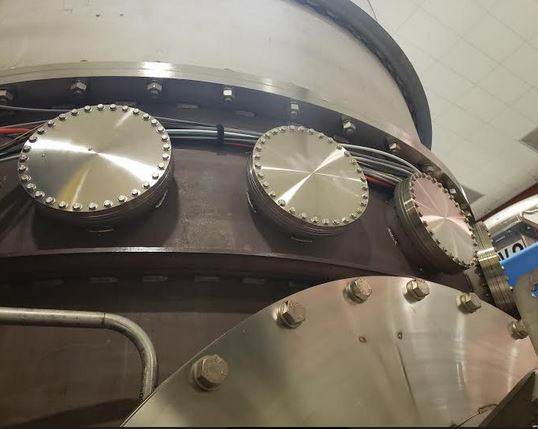
Removed cable tray baskets from BSC 7,8 to clear overhead for new door installation in Oct. as part of the H2 decoupling exercise. There were no cables in trays on BSC8. BSC7 (x-arm side) basket supported a bundle of cables that are temporarily draped over the large flanges above. See photo.
Per ECR E1900176, FRS 13051, WP 8364, measured the effect of moving the IO high power beam dump hoses. The largest changes were seen at 420Hz, 480Hz, and 550Hz, where the coherance peaks at those frequencies, between the PSL periscope Y accelerometor and the IMC WFS signal WFS A Yaw measured anywhere between 0 and 0.6. Of course there was no one hose position that minimized alll of the peaks, but the changes, with changing the hose locations, were easily identified.
Hose positions tried:
It was clear that there were outside influences to the measurements, and I suspect first and foremost the temperature of the PSL, so the coherance at 550Hz was low when we started, and high when we left, and I believe the coherance will decrease as the PSL temperature returns to steady-state Scinence Mode.
Plots will be added later.
- Jason, Cheryl
I reset both PSL power watchdogs at 20:21 UTC (13:21 PDT). This completes FAMIS 10729.
Matthew Ball, Dripta Bhattacharjee, Adrian Helmling-Cornell, Robert Schofield
Recent DQ shifts have noted that the H1:PEM-EX_ADC_0_17/18/19_OUT_DQ channels have started appearing in hveto (51515, 51759). Channel 17 measures the potential between the low-voltage ESD chassis and the beamtube. Channels 18 and 19 measure the voltage of the power supply for the ESD. We confirmed today that all three channels were set up properly, so it does not appear to be a wiring issue causing the glitching.
WP8376 h1tw1 raw minute trend disk almost full
Jonathan, Dave:
The workpermit was to investigate if we could temporarily use h1tw3's data for h1fw1 instead of the almost full h1tw1 data disk. We will be decommissioning h1tw1 in October and so we didn't want to go through with a full offload procedure if it could be skipped).
We tested this out initially on h1nds0 (only used by guardian) and found that the NDS1 code could not handle duplicate data (data in both the online raw_minute area and in the archived area).
So we are going to have to do a standard SSD->HDD offload.
h1nds0 was restarted twice (going into test mode, and then reverting back)
h1nds1 was restarted once (getting 5 months of raw minute from the frozen area on h1tw1's SSD while the data is being transferred).
I started the data transfer at 12:53 PDT, it normally takes about a day. h1tw1 disk is 96% full and I expect it to fill by the weekend.
While the work on the HAM5/6 work platform was happening this morning, a part fell and knocked a viewport cover off. This hit the corner 3 horizontal Parker valve cover, and dented the aluminum cover and left a bit of yellow paint. I'm posting an image of the damage to the Parker valve cover. It's not small, but there are no fluid leaks and the dents are on the edge of the casing. Hugh is running some tests, he should post those soon.
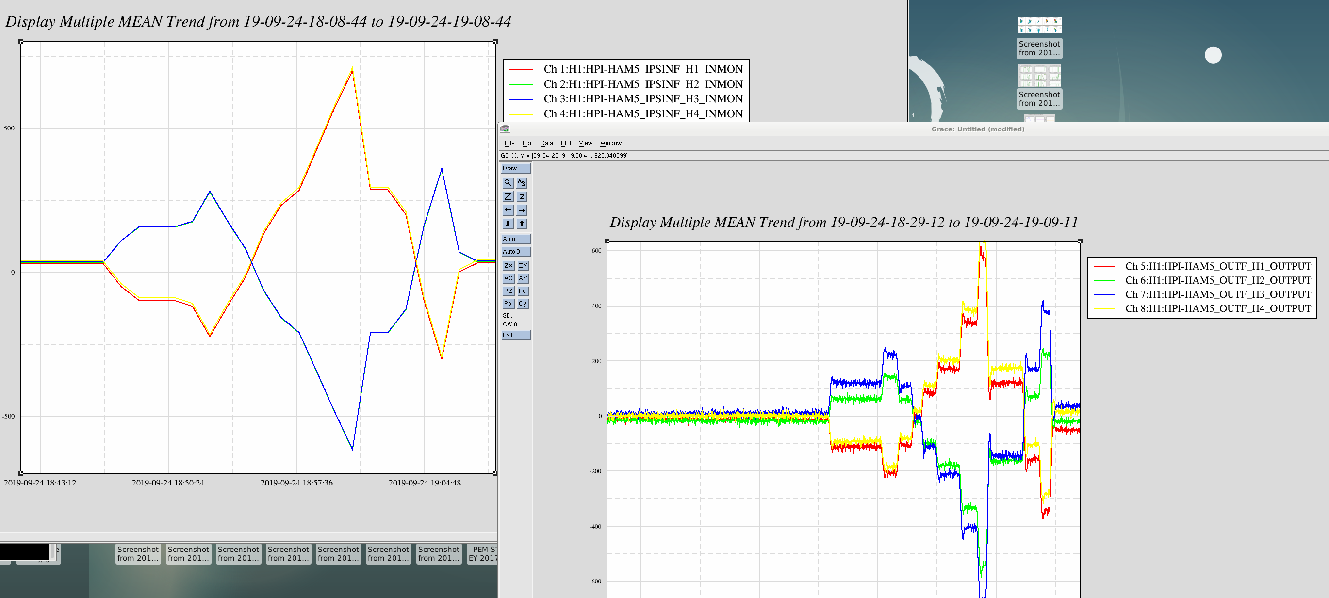
Here are a couple trend plots of the IPS position sensors and the output drives to the actuators while doing strokes on the Y dof of +- ~50um. The positions of the IPS suggest all the actuators are moving the same amount to achieve the cartesian displacement request. The output drives are not the same for the four corners but each corner may have its own resistance from nominal isolated position and its own force coeffiecient. HEPI remains functional here.
We have spare parker valves on the shelf and maybe this should be changed in October if for no other reason than to clean off the yellow paint.
Ops Shift Transition: 09/24/2019, Day Shift 15:00 – 23:00 (08:00-16:00) - UTC (PT)
State of H1: Tuesday Maintenance
Intent Bit: Commissioning
Weather: 0-5 mph wind
Primary 0.03 – 0.1Hz: 0.01 um/s
Secondary 0.1 – 0.3Hz: 0.3 um/s
Outgoing Operator: TJ
Quick Summary: Tuesday maintenance ongoing, crane work/VAC work started
TITLE: 09/24 Owl Shift: 07:00-15:00 UTC (00:00-08:00 PST), all times posted in UTC
STATE of H1: Preventive Maintenance
INCOMING OPERATOR: Niko
SHIFT SUMMARY: Quiet shift, locked for ~9 hours. A few earthquakes rolled through, but we held lock. PEM script was ran.
LOG:
I hadn't noticed that we were in Earthquake mode on my arrival, and then a notification for a 5.7 earthquake in Greece came in. After we rode through it, I brought it back to WINDY, but it was a rough transition. Made it though.
TITLE: 09/24 Owl Shift: 07:00-15:00 UTC (00:00-08:00 PST), all times posted in UTC
STATE of H1: Observing at 113Mpc
OUTGOING OPERATOR: Ed
CURRENT ENVIRONMENT:
SEI_CONF state: EARTH_QUAKE
Wind: 8mph Gusts, 7mph 5min avg
Primary useism: 0.02 μm/s
Secondary useism: 0.15 μm/s
QUICK SUMMARY: Fresh lock ar one hour, calm environment.
TITLE: 09/24 Eve Shift: 23:00-07:00 UTC (16:00-00:00 PST), all times posted in UTC
STATE of H1: Observing at 114Mpc
INCOMING OPERATOR: TJ
SHIFT SUMMARY:
LOG:
23:00 Dan B out o the Optics Lab
23:30 Intention bit Commissioning - PEM team
00:31 H1 back to Observing - PEM team back
J. Kissel
H1 has been using the same reference DARM loop calibration model parameter set for all of O3 thus far (modelparams_H1_20190416.py). However, much has changed with the IFO and our understanding of it since then, and it's time to update. This aLOG describes why we're (finally) updating, what we've updated to, using what data sets, the new associated uncertainty it will bring, and all the scripts, process, and effort to make the self-consistent new parameter set and uncertainty (one person, two 16 hours days, an answer 3 days *before* installation -- record time!). The model will be installed, and the calibration will be updated on Monday, 2019-09-09, with the installation to begin around 9:30a PDT and will take effect the next indicated observation /analysis ready segment (don't worry, once that segment has started and its start time known, I'll be sure to communicated that far and wide).
Why: Here're the major things that have changed:
(1) We've increased our laser power in to the IFO from "35 Watts" to "37 Watts" (see LHO aLOG 51734 for discussion of why I put those numbers in quotes) on Jun 10th. However, we contested that because our time-dependent correction factors (TDCFs) are correctly capturing them, and we're correcting for them down-stream in our low-latency h(t) production (aka GDS-CALIB_STRAIN), (and (2) was still happening) it was not worth the effort to update the front-end calibration (aka DELTAL_EXTERNAL). This meant that \kappa_C (the correction for optical gain change, say, due to laser power increase) has been perpetually ~0.96 %, which results in the niggling discrepancy we've seen on the Inspiral Range Figures of Merit comparing "the answer" from the two data streams (see e.g. the summary page plot from today).
(2) We've drastically reduced the amount of confusion that we've had with the low frequency, opto-mechanical response (aka the sensing function) of the detector by installing a digital, length offset in the signal recycling cavity, and thus reducing the detuning of the cavity that we've had (the so called permanent 100 ct SRCL offset; see LHO aLOG 51592). This offset also has slightly improved / increased our DARM coupled cavity pole frequency. Still some confusion remains, but little enough that we don't think we need to include static compensation for detuning in our model of the sensing function, taking the hit terms of an unknown systematic error. This error is significantly less than what we've ascribed previously (see conclusions in for data up through August in G1901479). Further, we've found that our MCMC algorithm can handle the data again, which means we no longer have to use a model that barely represents what we measure, and we can again have a self-consistent uncertainty budget.
(3) We found a way to re-install PUM L2A decoupling filters, reducing global ASC motion (have our cake, see LHO aLOG 51604) and with a new topology (LHO aLOG 49825), it no longer creates parasitic L2A2L, low frequency distortions of the PUM's L drive to TST L displacement (and it eat it too, see LHO aLOG 51782 and references therein)
(4) We've found a small change in the actuation authority distribution, a boost of a factor of ~3 at 0.2 Hz, tapering off to a factor of 2-ish below that on the UIM stage (see LHO aLOG 51740), relieving some control from the PUM stage, which may have caused some lock losses due to saturation.
With these cumulative changes, and a model that matches our data self-consistently, it's time we update the calibration in the front-end and improve the accuracy of our low-latency data.
What, How, What Data Sets, Process, and Cognizent Decisions Along the Way:
The new model parameter set lives here:
^/trunk/Runs/O3/H1/params/modelparams_H1_20190909.py rev 8365
The only things that differ from the previous model,
^/trunk/Runs/O3/H1/params/modelparams_H1_20190416.py rev 7237
are the some of the optical response "sensing function" parameters, which are now
# (from MCMC fit of 2019-09-04 'nominal config' data, restricted to above 20 Hz)
ccOpticalGain = 3.181e+06 #cnts/meter
ccPoleFreq = 411.2929 #Hz
detuneSpringFreq = 0.0 #Hz MCMC fit is 0.13 Hz, but consistent with zero so install no detuning frequency.
detuneSpringQ = 1e-2 # MCMC fit is 1.87, but consistent with no spring, so install no detuning Q.
# *Rough* Conversion from DARM IN1 [ct] to Current on DCPDs [mA]
# Transfer function magnitude H1:OMC-DCPD_SUM_OUT_DQ/H1:LSC-DARM_IN1_DQ (entirely digital, but needs to be in NLN data stretch)
# 5 Hz value at "start" time from above, 25 avgs, 0.1 Hz binwidth DTT FFT
omcdcpdout2darmin1tf = 1.362605e6 # Mean of 2019-08-21, 2019-08-28, and 2019-09-04 values, std(values)=0.07% >> doesn't change appreciably.
# GDS Compensation for Bad Foton Filter Approximation for 7 kHz High Frequency Roll-Off of 1/C
# (from MCMC fit of 2019-09-04 'nominal config' data, restricted to above 20 Hz)
# O3B_D2N = zpk([413.5227],[7000],1,"n")
# O3B_Gain = gain(3.149e-07)
CfotonInvSensingTF = SVNROOT+'trunk/Runs/O3/H1/Measurements/Foton/2019-09-09_H1CALCS_InverseSensingFunction_Foton_SRCD-2N_Gain_tf.txt' #export
and on the actuator side, the filter file and what's in use from that filter file for ETMX on the UIM (L1) stage
AfilterFile_X = SVNROOT+'trunk/Common/H1CalFilterArchive/h1susetmx/H1SUSETMX_1251574934.txt' # Sep 03 2019 19:41:56 UTC
UIMlockName = 'ETMX_L1_LOCK_L'
UIMlockModules = [2,10] # Here's the new UIM Boost "muBoost" in FM2. JSK 2019-09-05, see LHO aLOG 51709
UIMlockGain = 1.06
I'll start with the actuator, 'cause there hasn't been much change there: as discussed in LHO aLOG 51782, we see no change in frequency response of the any of the three stages of SUS ETMX used for DARM control, UIM (L1), PUM (L2), or TST (L3) as a result of either of the changes (3) or (4) above. Thus, all we need to do here, is update the copy of the foton file, and let the model know to use that new filter.
As bonus, that means several things for the uncertainty / systematic error estimate for the actuator:
(a) We don't need to update the actuation strength estimate, so we can use the same values and MCMC posterior distributions of uncertainty on these parameters that we've been using all along throughout O3. Much less work! Good! We'll continue to use
HDF5_A_MCMCresults=/ligo/svncommon/CalSVN/aligocalibration/trunk/Runs/O3/H1/Results/Uncertainty/O3_H1_A_MCMC_20190404.hdf5 rev 7476
(b) We can just lump these latest measurements into our collection of data sets that inform the unknown systematic errors in frequency dependence for each stage. With these new data sets, the uncertainty on that unknown systematic error will improve.
(c) With the new found better understanding of where to restrict the frequency range of MCMC fit, and how to use the Gaussian Process Regression fitting tool to estimate that unknown systematic error (see G1901479, and discussions of length scale and frequency range), we can refine our estimate further.
All that culminates in a new and improved uncertainty estimate (from the improved uncertainty in unknown systematic error) for the actuator.
The script I used that produce the updated unknown systematic error estimate is
^/trunk/Runs/O3/H1/Scripts/Uncertainty/process_allmeas_writeGPRHDF5_model20190909-A.py rev 8389
See the first six .pdf attachments, 2019-09-04_H1_???_actuationMeasurement_allresiduals_MCMCInput.pdf and H1_model2019-09-09_meas2019-09-04_???_actuationMultiGPR.pdf which show the collection of measurements used (first set), and the resulting fit for unknown systematic error (second set).
Now to the more complicated part: the changes in sensing function parameters and their associated parameter uncertainty, and contribution to response function uncertainty.
(a) We've collected, now, 4 data sets in the current sensing function configuration: the restored "July" spot positions, and *with* a digital 100 ct SRCL offset: 2019-08-21, 2019-08-28, and now two data sets that turned out to be not that different on 2019-09-04. Like Evan did for his update of the uncertainty for C01 (again see G1901479), I asked -- "how different of parameter answers and/or goodness do we get if we MCMC over the entire frequency span of the data set, or just restrict it frequencies which we believe can be well-explained by our model?" After looking at 8 different MCMC results -- a fit range of 5 to 5000 or 20 to 2000 for all 4 data sets -- I came to the conclusion that a lower limit of 20 Hz gave better, more consistent results AND for the following reasons, I used the 2019-09-04 "nominal config" (i.e. no PUM L2A decoupling and UIM boost OFF) :
- Gives best results for MCMC fit (small frequency-dependent residuals between fit and measurement)
- Gives "middle of the road" f_cc, and f_s values (comparing the answers from all the >20 Hz data)
- Optical gain is with the 0.5% variance of all fit answers for optical gains
- f_s values are all consistent with zero, so OK to choosing to enter 0 Hz (no) spring in foton, and install model with 0 Hz (i.e. no) detuned spring.
- Intentionally not using averaging of all dates, because we need to have representative MCMC posteriors for each parameter to have self consistent model and implementation.
The results for that fit on the 2019-09-04 nominal config data, with 20 > f_fitRange > 5000 are
Optical gain, H_c (ct/m) | 3.181e+06 (+ 958,-958.7) or (+0.03012%,-0.03014%)
Optical gain, H_c (mA/pm) | 4.334 (+0.001305,-0.001306) or (+0.03012%,-0.03014%)
Cavity pole, f_cc (Hz) | 411.2929 (+0.7354,-0.7224) or (+0.1788%,-0.1756%)
Detuned SRC spring frequency, f_s (Hz) | 0.1345 (+0.1005,-0.04764) or (+74.75%,-35.43%)
Detuned SRC spring quality factor, Q_s | 1.872 (+3.464,-4.302) or (+54.05%,-43.52%)
Residual time delay, tau_c (usec) | -1.252 (+0.4738,-0.4692) or (+-37.83%,--37.46%)
and thus the chosen parameter values. I'll highlight that the f_s value is consistent with zero, so I've chosen to install model parameters that force no detuning.
The two attachments 2019-09-04_H1_fmin20Hz_sensingFunction_mcmcModel_vs_measurement.pdf and 2019-09-04_H1_fmin20Hz_sensingFunction_mcmcModel_paramCornerPlot.pdf show the MCMC fit and the corresponding posterior distribution corner plot for 2019-09-04, "nominal config" data.
(b) The script to process that particular fit and save the posterior distribution on those parameters is
/ligo/svncommon/CalSVN/aligocalibration/trunk/Runs/O3/H1/Scripts/FullIFOSensingTFs/
process_sensingmeas_20190904_nomconfig.py rev 8368
which spits out (upon request, I've relearned by calling an extra function writeSensingMCMCposteriorsHDF5 from /ligo/svncommon/CalSVN/aligocalibration/trunk/Common/pyDARM/computeDARM.py src7213) an .hdf5 file recording the posteriors here
/ligo/svncommon/CalSVN/aligocalibration/trunk/Runs/O3/H1/Results/Uncertainty
O3_H1_C_MCMC_20190904_nomconfig_fmin20Hz_finaltrial.hdf5 rev. 8364
I re-learned the hard way that these need to be done once you like the results of the MCMC fit -- and sadly, sometimes the fit gives irreproducible results, so if you get one set of a parameter answers you like one day, then come back the next and actually write the answers to file, your MAP values may be inconsistent -- especially if the posterior distribution is non-Gaussian like we have!
(c) Armed with a set of Maximum A-Posteriori (MAP) values, I can then update the model parameter set (see above), AND also generate the export of foton's bad approximation to the near-nyquist 7000 Hz pole necessary to roll off the inverse sensing function filter that gets installed in the front-end, hence,
/ligo/svncommon/CalSVN/aligocalibration/trunk/Runs/O3/H1/Measurements/Foton/2019-09-09_H1CALCS_InverseSensingFunction_Foton_SRCD-2N_Gain_tf.txt
NOTE: the MCMC fit analysis code assumes we'll be using the MAP values, so it gave me the following foton design string to install and export:
SRCD2N: zpk([411.2929;0.1033;-0.1751],[0.1;0.1;7000],1,"n")gain(1.81)
Gain: gain(3.144e-07)
However, because as discussed in (a) I've intentionally installed NO detuning in the model, so I instead used the following design string for the export:
zpk([411.2929],[7000],1,"n")
(d) Finally, given that we have 4 data sets of the sensing function in the same configuration, it makes sense to estimate the unknown systematic error -- i.e. make sure we cover what's left over of the confusing low-frequency response as an element to our response function uncertainty. So I collected the afore mentioned 4 data sets and played the GPR fitting parameter game until I was satisfied, using the following script:
/ligo/svncommon/CalSVN/aligocalibration/trunk/Runs/O3/H1/Scripts/Uncertainty/
process_allmeas_writeGPRHDF5_model20190909-C.py rev 8370
and saved the results to
/ligo/svncommon/CalSVN/aligocalibration/trunk/Runs/O3/H1/Results/Uncertainty/
O3_H1_C_GPR_20190909_multi_nofsQcorr_fmin20Hz_lengthscaleZp5.hdf5 rev. 8371
The collection of data compared against the new model is shown in attachment 2019-09-04_H1_20190909Model_sensingFunction_referenceModel_vs_allMeasurements.pdf and the GPR fit for it is H1_allO3BMeas_nofsQcorr_fmin20Hz_lengthscaleZp5_model2019-09-09_meas2019-09-04_sensingFunction_GPR.pdf.
Oooooh kay! Kudos to you if you've even made it this far in the reading. #kLOG.
Associated Uncertainty
Now, armed with the actuation function's parameter uncertainty and unknown systematic error with its associated uncertainty, and the same for the sensing function, we can produce a response function uncertainty, using
/ligo/svncommon/CalSVN/aligocalibration/trunk/Common/pyDARM$
RRNom.py rev 8377
This is unfortunately a function, in which the list of arguments is longer than my arm, so I'll explicitly report it here for future reference (the python3 part is necessary):
python3 RRNom.py --IFO=LHO --HDF5_A_MCMCresults=/ligo/svncommon/CalSVN/aligocalibration/trunk/Runs/O3/H1/Results/Uncertainty/O3_H1_A_MCMC_20190404.hdf5 --HDF5_A_GPRresults=/ligo/svncommon/CalSVN/aligocalibration/trunk/Runs/O3/H1/Results/Uncertainty/O3_H1_A_GPR_20190909_multi.hdf5 --HDF5_C_MCMCresults=/ligo/svncommon/CalSVN/aligocalibration/trunk/Runs/O3/H1/Results/Uncertainty/O3_H1_C_MCMC_20190904_nomconfig_fmin20Hz_finaltrial.hdf5 --HDF5_C_GPRresults=/ligo/svncommon/CalSVN/aligocalibration/trunk/Runs/O3/H1/Results/Uncertainty/O3_H1_C_GPR_20190909_multi_nofsQcorr_fmin30Hz_lengthscaleZp5.hdf5 --modelPath=/ligo/svncommon/CalSVN/aligocalibration/trunk/Runs/O3/H1/params/ --modelFilename=modelparams_H1_20190909 --IFOmodel=modelPars --outDir=/ligo/svncommon/CalSVN/aligocalibration/trunk/Runs/O3/H1/Results/Uncertainty/ --plot1SigmaUncs --plotSamplesAndUncs --sampleNumber=1000 --seed=1234 --version=ref --saveSummaries --gpsTime=1251687618 --PcalSweepData=/ligo/svncommon/CalSVN/aligocalibration/trunk/Runs/O3/H1/Measurements/FullIFOSensingTFs/2019-09-04_H1_NominalConfig_PCAL2DELTAL_LF_SS_A_PCALYRX_B_DELTALEXT_tf.txt --GetData=GWPY
There's probably some parts of this I don't need, but I was follow as best I could from the README here:^/trunk/Common/pyDARM/README rev. 8379
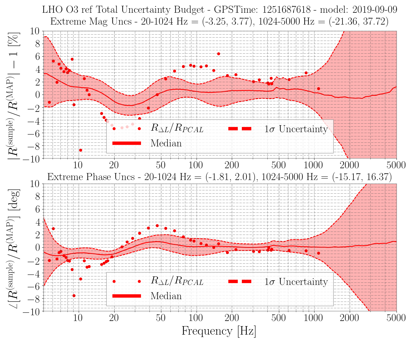
The results are the only image attachment, 2019-09-06_O3_LHO_GPSTime_1251687618_ref_RelativeResponse1SigmaUncertainty.png.
One can see that the maximum 68% ci bounds of the frequency region from 20-1024 Hz on the response function uncertainty and systematic error are 3.77% and 2.01 degrees.
This is better than reported for C01 at the start of O3 through Jun 11th, over a similar frequency range -- most-notably around 20-30 Hz where we've reduced the uncertainty in (i) unknown systematic error for the sensing function by improving the low frequency response, i.e. reducing the SRC detuning, and (ii) unknown systematic error for the actuation function by adding more measurements and improving the Gaussian process regression parameters.
for this reference model (remember, doesn't include the uncertainty of time-dependent correction factors determined from calibration line coherence)
Attached are all the plots that show the supporting data.
The plots live in the following locations in the repo (worth it to record here, because the results directories can be a mess of trials and errors), in order of attached list:
^/trunk/Runs/O3/H1/Results/Uncertainty/
2019-09-04_H1_UIM_actuationMeasurement_allresiduals_MCMCInput.pdf
2019-09-04_H1_PUM_actuationMeasurement_allresiduals_MCMCInput.pdf
2019-09-04_H1_TST_actuationMeasurement_allresiduals_MCMCInput.pdf
^/trunk/Runs/O3/H1/Results/FullIFOSensingTFs/
2019-09-04_H1_20190909Model_sensingFunction_referenceModel_vs_allMeasurements.pdf
^/trunk/Runs/O3/H1/Results/Uncertainty/
H1_model2019-09-09_meas2019-09-04_UIM_actuationMultiGPR.pdf
H1_model2019-09-09_meas2019-09-04_PUM_actuationMultiGPR.pdf
H1_model2019-09-09_meas2019-09-04_TST_actuationMultiGPR.pdf
^/trunk/Runs/O3/H1/Results/FullIFOSensingTFs/
2019-09-04_H1_fmin20Hz_sensingFunction_mcmcModel_vs_measurement.pdf
2019-09-04_H1_fmin20Hz_sensingFunction_mcmcModel_paramCornerPlot.pdf
^/trunk/Runs/O3/H1/Results/FullIFOSensingTFs/
2019-09-04_H1_20190909Model_sensingFunction_referenceModel_vs_allMeasurements.pdf
^/trunk/Runs/O3/H1/Results/Uncertainty/
H1_allO3BMeas_nofsQcorr_fmin20Hz_lengthscaleZp5_model2019-09-09_meas2019-09-04_sensingFunction_GPR.pdf
^/trunk/Runs/O3/H1/Results/Uncertainty/
2019-09-06_O3_LHO_GPSTime_1251687618_ref_RelativeResponse1SigmaUncertainty.png
2019-09-06_O3_LHO_GPSTime_1251687618_ref_RelativeResponseUncertaintyBudget.png
2019-09-06_O3_LHO_GPSTime_1251687618_ref_RelativeResponseUncertainty_FinalResults.txt
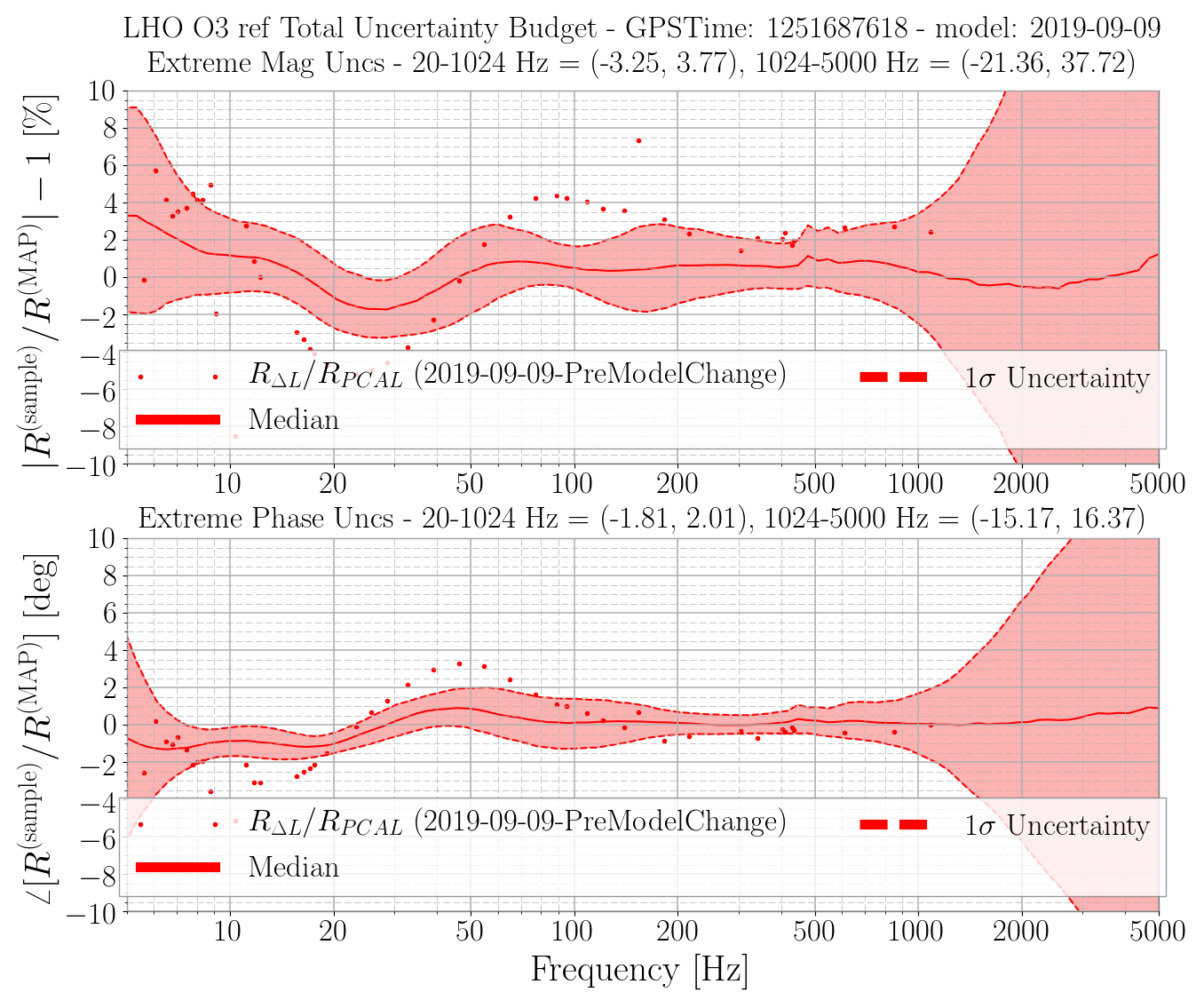
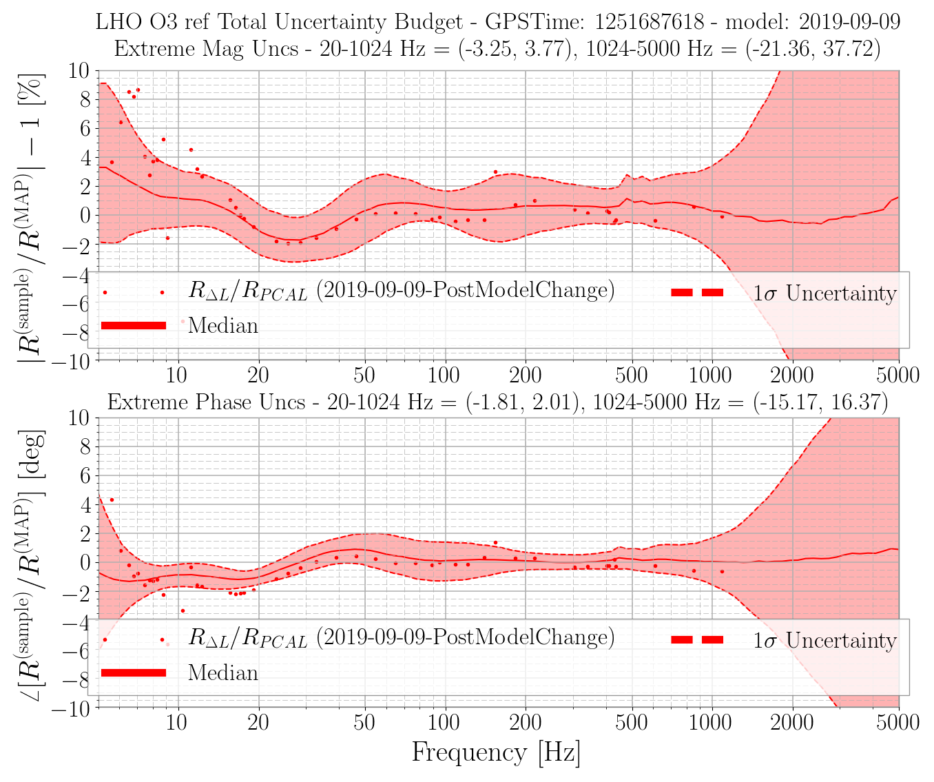
In the original alog, we see that the PCAL2DeltaL measurements do not agree with the envelope on the uncertainty plot. This is because the measurement was taken after the IFO changed but before the model was applied, i.e., the "Delta L" was not updated. Please see the three attached uncertainty plots with three sets of PCAL2DeltaL measurements: 0909PreModelChange, 0909PostModelChange, and 0916. It is clear that after the model change, the measurements 0909PostModelChange and 0916 both agree with the uncertainty envelope, but the one before the model change, 0909PreModelChange, does not agree with the envelope.
These plots are committed to ^trunk/Runs/O3/H1/Results/Uncertainty/PCAL2DARMvsUnc/
The command lines used to produced these plots are in ^trunk/Runs/O3/H1/Results/Uncertainty/PCAL2DARMvsUnc/commands.txt
J. Kissel In order to assess its time-dependence, and to go a little bit further to confirm the effect, we repeated last week's measurement of the DARM sensing function's low-frequency response to SRCL offset (see LHO aLOG 51440), this time with a SRCL offset of - 0 ct (what we've been running with since O3 started), - 100 ct, and - today, newly 200 ct (we lost lock 3/4s of the way through the measurement suite, but enough to salvage the data) to make some definitive conclusions and decisions about it. %%%% Executive Summary%%%% We installed a 100 ct digital offset in the SRCL loop, and modified the ISC_LOCK guardian to turn it on during the LOWNOISE_LENGTH_CONTROL state; it succeeded, and we've accepted it into the OBSERVE SDF. This improves the low-frequency sensing function by reducing the detuned SRC optical spring effects, reducing the complexity of the DARM response to displacement. We have not yet updated the calibration to reflect this, and I think we may not have to. Also, more details later (see point 5 below), but just so we're no longer sad about the physical interpretation of this digitally requested, I give you my crude calibration for the digitally requested SRCL offset: Digital SRC Phase SRC Length 0 ct = - 0.34 (+/- 0.02) deg = - 57.6 (+/-3.4) nm 100 ct = + 0.00 (+/- 0.01) deg = 0.0 (+/-1.7) nm 200 ct = + 0.28 (+/- 0.02) deg = + 47.4 (+/-3.4) nm (with dl- = [ lambda / (2*pi) ] * phase, and lambda = 1064e-9 m) %%%% DETAILS and FIGURES %%%% Here're the conclusions: (1) A requested digital SRCL offset of 100 ct can repeatedly reduce the amount of detuning seen in the DARM sensing function -- however, what's left over is still time-dependent. See first attachment: 2019-08-28_H1_SRCLOffsetTest_Jul100ct_sensingFunction_referenceModel_vs_allMeasurements.pdf This compares last week's and this week's measurements in the pre-August spot positions against a model. As in previous aLOGs, I divided the measurement by an hand-tuned sensing function model with no optical spring, in order to show / expose what response is down there, since we know we can't attribute the response entirely to just SRC detuning; some parasitic L2A2L coupling remains. And indeed, we can't disentangle whether it's the parasitic L2A2L or the SRC detuning that's time dependent. This hand-tuned model parameter set: /ligo/svncommon/CalSVN/aligocalibration/trunk/Runs/O3/H1/params/ modelparams_H1_20190416_byopticalresponseforjulspot100ctSRCLoffset.py which only differs from the nominal O3 model in - lack of optical spring (detuneSpringFreq = 0.0), - the optical gain (ccOpticalGain) is 3.16e6 (corresponding to a \kappa_C of 0.972, as expected from the lack of updating for power up from 35W to 37W), and - the cavity pole frequency (ccPoleFreq) is 417.0 Hz but at least, (yes, only a sample size of 2), we conclude the low-frequency response is still time dependent with a 100 ct offset, but not by much. (2) While we lost lock halfway through the PCAL2DARM sweep, I had a full DARM Loop Suppression measurement in the can during the time which the IFO had a requested digital SRCL offset 200 ct. Thankfully this is enough data to resolve the low-freqnecy response. See second attachment: 2019-08-28_H1_SRCLOffsetTest_OffsetComp_sensingFunction_referenceModel_vs_allMeasurements.pdf This compares the three measurements of the above mentioned offsets. One can clearly see that between a digital offset of 0 to 200 ct, we're flipping between an pro-spring (0 ct offset) an anti-spring (200 ct offset), and some how, miraculously 100 ct offset lands use pretty darn close to perfectly tuned. However, as is seen in the first and now the second plots -- at 100 ct, there remains some for of stuff going on. We'll blame it on parasitic L2A2L, so we won't for now, try to find the "perfect" SRCL offset, and continue down the Sheila / Matt path of trying to crush the parasitic L2A2L. From these two plots, we conclude that a 100 ct SRCL offset is good, and we'll now stick permanently with it. (3) Now -- what does this mean for the calibration? See third attachment: 2019-08-28_H1_SRCLOffsetTest_Jul100ct_NomModel_sensingFunction_referenceModel_vs_allMeasurements.pdf Here, I show the currently installed reference model against the two data sets we have with the July spot positions, but with a 100 ct SRCL offset. - We already know the optical gain is too high at 3.25e6 ct/m, but that's covered by \kappa_C at 0.97. - We already know that the cavity pole is a bit too low at 411, but that's covered by f_cc which nicely is reporting 418 Hz or so at the beginning of a nominal lownoise stretch after power-up, and settles in to about 414 Hz after thermalization. - So it's only the low-frequency response that should concern us: since there's essential no detuning at a 100 ct SRCL offset, the current model, which has a pro-spring of 4.47 Hz, gives as much as 4% systematic error at 20 Hz, and 14% error at 10 Hz. BUT -- as Evan inadvertently shows in the Action Item Follow-up Slides of G1901479, if we have a systematic error in the sensing function (as represented by the 68% CI shaded region), then it's not until that error starts getting about a factor of 2 worse -- ~8% at 20 Hz (25-30% at 10 Hz) -- that we really start to spoil the systematic error of the entire response function. So I think we're OK here. The resulting low-frequency systematic error created by improving the sensing function reality without updating the calibration model of it is smaller than other dominant overall response function systematic errors and uncertainties in this frequency region. I wouldn't be opposed to creating a new reference model starting with this data set, but there's *a lot* of things to remember to do besides just updating the front-end model (see, e.g., an incomplete list here: T1800469.) (4) What if we went forward with our existing techniques and pushed a new model that is derived from the MCMC fit infrastructure we have? See fourth and fifth attachment: 2019-08-28_H1_SRCLOffsetTest_Jul100ct_NomModel_sensingFunction_mcmcModel_vs_measurement.pdf 2019-08-28_H1_SRCLOffsetTest_Jul100ct_NomModel_sensingFunction_mcmcModel_paramCornerPlot.pdf The MCMC puts forth a pretty solid fit, with Optical gain, H_c (ct/m) | 3.159e+06 (+1041,-959.4) or (+0.03297%,-0.03037%) Cavity pole, f_cc (Hz) | 419.8 (+0.7607,-0.8149) or (+0.1812%,-0.1941%) Detuned SRC spring frequency, f_s (Hz) | 2.152 (+0.02577,-0.02861) or (+1.198%,-1.33%) Detuned SRC spring quality factor, Q_s | 97.36 (+2007,-4929) or (+4.85%,-1.975%) Residual time delay, tau_c (usec) | 1.987 (+0.4861,-0.5282) or (+24.46%,-26.58%) which is consistent with my by-hand fit, has .... let's say 1-2% / 2 deg scatter level systematic error down to at least 7 Hz, and only has a few walkers in parameter "islands." I would be comfortable attributing the rest of the systematic error to the parasitic L2A2L coupling, and moving on without having to worry about a detuned spring anymore. Plus -- if Sheila / Matt are getting closer to trying out their L2A decoupling, then maybe this secondary effect will also disappear... I'm getting ahead of myself though. I've gotta sleep on this (and we've gotta replace an HEPI pump tomorrow), but stay tuned for a decision on whether to update the reference model. (5) The promised details on the calibration of the SRCL offset: This calibration / fit to the data uses the very handy Cahillane DARM Plant interactive plotter python script from LHO aLOG 48366, updated for an input power of 36.8 W, with a PRG of 45, and (perhaps incorrectly, oddly the data demands that) the SRM transmission is 36.05% (where "we know" that the SRM has been replaced with SRM-06 Post O2, which galaxy, says LIGO measured 32.34%, but the report is empty, and the vendor data sheet says 31.80%). I agree that (a) I've probably done something wrong, (b) that the physical values for the detuning appear to be an order of magnitude larger than what they were in O1/O2 (see LHO aLOG 27675) so forgive me for now while I still try to get an understanding of how the calibration of this offset works. *I've* done nothing complicated -- Craig has done all the work for me of making the amazing tool which converts physical parameters into a sensing function -- and gives you interactive control over the important ones that influence the shape of the response function. So -- that's what I did. Eyeballed the fits (with the above state precision), and came up with that kind of SRC phase. See sixth attachment: 2019-08-28_H1DARM_SensingFunction_CraigModel.pdf This shows three pages for the three measurements with three different offsets. Virtually all physical parameter values are kept at their nominal measured values, except for -- as mentioned above -- the SRM transmission. (well, and yes, OK, there's a 0.07 log-scale correction to the optical gain, but optical gain loss could be anything). Importantly though -- between the three fits, I only varied the SRC detuning phase. Anyways -- more to sleep on.

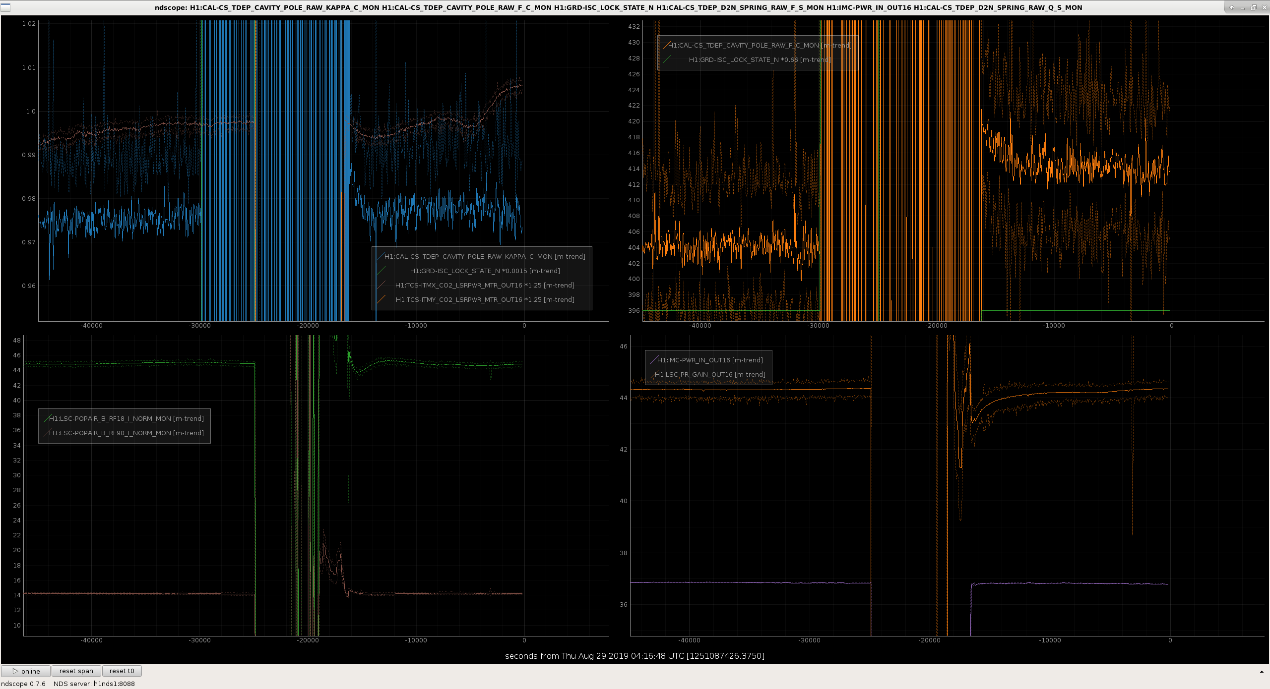
Just a quick *before* vs. *after* (the application of the 100 ct offset) trend of \kappa_C and f_cc between the previous nominal_low_noise / observation segment and this one. The cavity pole frequency is now back to Mar 2019 levels in the ~415 Hz region! Also -- you'll note that before the soft loops / ADS settle -- which, PS, still takes on the order of an hour or two (why??) -- we hit the nominal low noise segment with a cavity pole of 420 Hz, and a nicely high optical gain, but it drops from there... PRC gain is about the same. POP18 / POP90 build-ups are about the same. "thermalized" / "ads converged" optical gain is about the same.
The first observation ready segment that permanently employed this new SRCL offset started at GPS 1251071403 (aka Aug 28 2019 23:49:45 UTC; Aug 28 2019 16:49:45 PDT).
With help from Stuart Aston at LLO and RahulK, BetsyW, JeffK, and EdM at LHO, this entry documents our current best understanding of the suspended masses of the ETMs.
Note that the Photon Calibrators generate calibrated forces on the ETMs via radiation pressure. The overall uncertainty of the actuation forces is below 1%, closer to 0.5% for the observing run.
To accurately translate these calibration forces into calibrated displacements, we require accurate masses of the suspended ETMs. A 0.1% error in the suspended mass directly couples into a 1% error in the calibrated displacements.
Here is what we know:
LHOx - 39611 grams
LHOy - 39538 grams
LLOx - 39508 grams
LLOy- 39642 grams
44 grams (2 x 22 grams)
The total mass of AMD1, 2, 3 and 4 is 0.80gm, 0.54gm and 0.39gm and 0.32gm respectively.
Total: 2.05 g
Rahul looking into this issue.
So our current best guesses for the masses are (neglecting the fibers for now):
LHO EX: 39611 + 44 + 2.05 = 39657 g
LHO EY: 39538 + 44 +2.05 = 39584 g
LLO EX: 39508 + 44 +2.05 = 39554 g
LLO EY: 39642 + 44 + 1.78 = 39688 g (Missing one AMD)
h1etmx.m
pend.m3 = 39.603+ear_mass_total; % 39.647 = 39.603 + ear_mass_total; Updated on 7 Aug 2015 by K.Izumi, ETM 08 on https://galaxy.ligo.caltech.edu/optics/. +0.044 from Betsy to include ear weight.
h1etmy.m
pend.m3 = 39.597 + ear_mass_total; % 39.641 = 39.597 + ear_mass_total; Updated on 12 feb 2014 by Brett Shapiro, ETM 12 (H1ETMY) on https://galaxy.ligo.caltech.edu/optics/.
l1etmx.m
pend.m3 = 39.508 + ear_mass_total; % 39.552 = 39.508 + ear_mass_total; Updated on 15 Feb 2019 by Stuart Aston, old ETM 07 new ETM 10 (L1ETMX) on https://galaxy.ligo.caltech.edu/optics/.
L1etmy
pend.m3 = 39.642 + ear_mass_total; % 39.686 = 39.642 + ear_mass_total; Updated on 15 Feb 2019 by Stuart Aston, old ETM 09 new ETM 15 (L1ETMY) on https://galaxy.ligo.caltech.edu/optics/.
Thus the masses in the suspension models as of May 22, 2019 seem to be (models may not be including the 2 g from the AMDs):
LHO EX: 39603 + 44 + 2.05 = 39649 g
LHO EY: 39597 + 44 +2.05 = 39643 g
LLO EX: 39508 + 44 +2.05 = 39554 g (was 39552 +46 = 39598 until 2/15/2019)
LLO EY: 39642+ 44 +1.78 = 39688 g (was 39686+46 = 39732 until 2/15/2019)
Summary
H1ETMX
Current model value 39649 g, should be 39657 g, error: model 8 g lighter than actual (0.02%)
H1ETMY
Current model value 39643 g, should be 39584 g, error: model 60 g heavier than actual (0.15%)
L1ETMX
Current model value 39554 g (correct value)
L1ETMY
Current model value 39688 g, was 39732 g until Feb 15, 2019, error: model 44 g lighter than actual (0.11%)
Theoretically, I estimated that each fused silica fibres should have a mass of about 0.494 grams, however if we consider around half of the fibre bending (when pendulum swings) then it should be around 0.247grams. Making a total of 0.988 grams for all four fibres.
If we want more precision, then it is better to take into account the actual bending length (which should around 20 mm from the top of the fibre). This should be around 0.172 grams (0.688 grams for all 4 fibres).
Seems there is a typo in what I wrote earlier.
"A 0.1% error in the suspended mass directly couples into a 1% error in the calibrated displacements." should have been "A 0.1% error in the suspended mass directly couples into a 0.1% error in the calibrated displacements."