jeffrey.kissel@LIGO.ORG - posted 12:51, Tuesday 26 August 2025 - last comment - 13:37, Tuesday 26 August 2025(86578)
H1 SUS PR3 Pitch and Yaw Estimator: Installed and Run for 1 hour
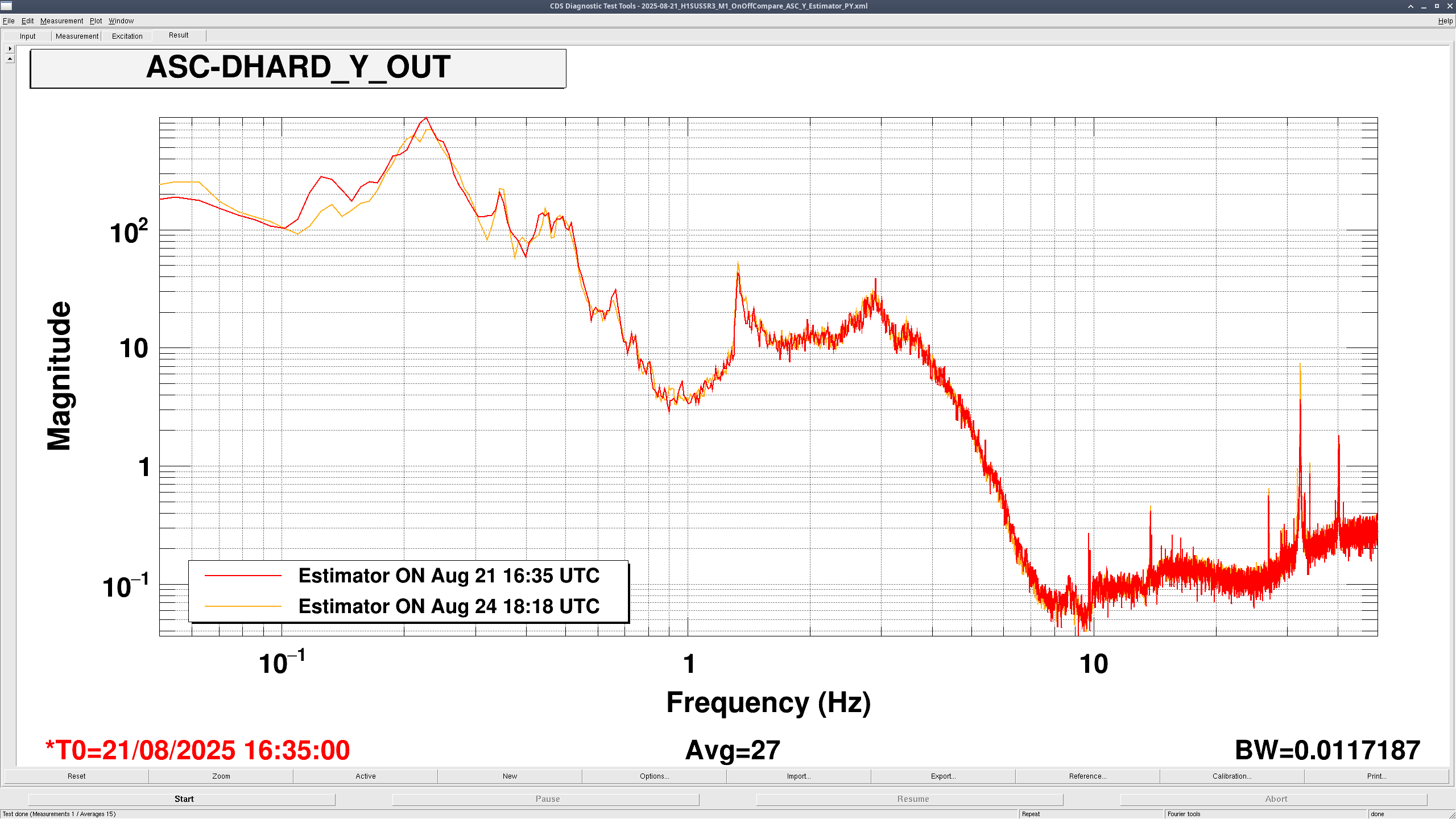
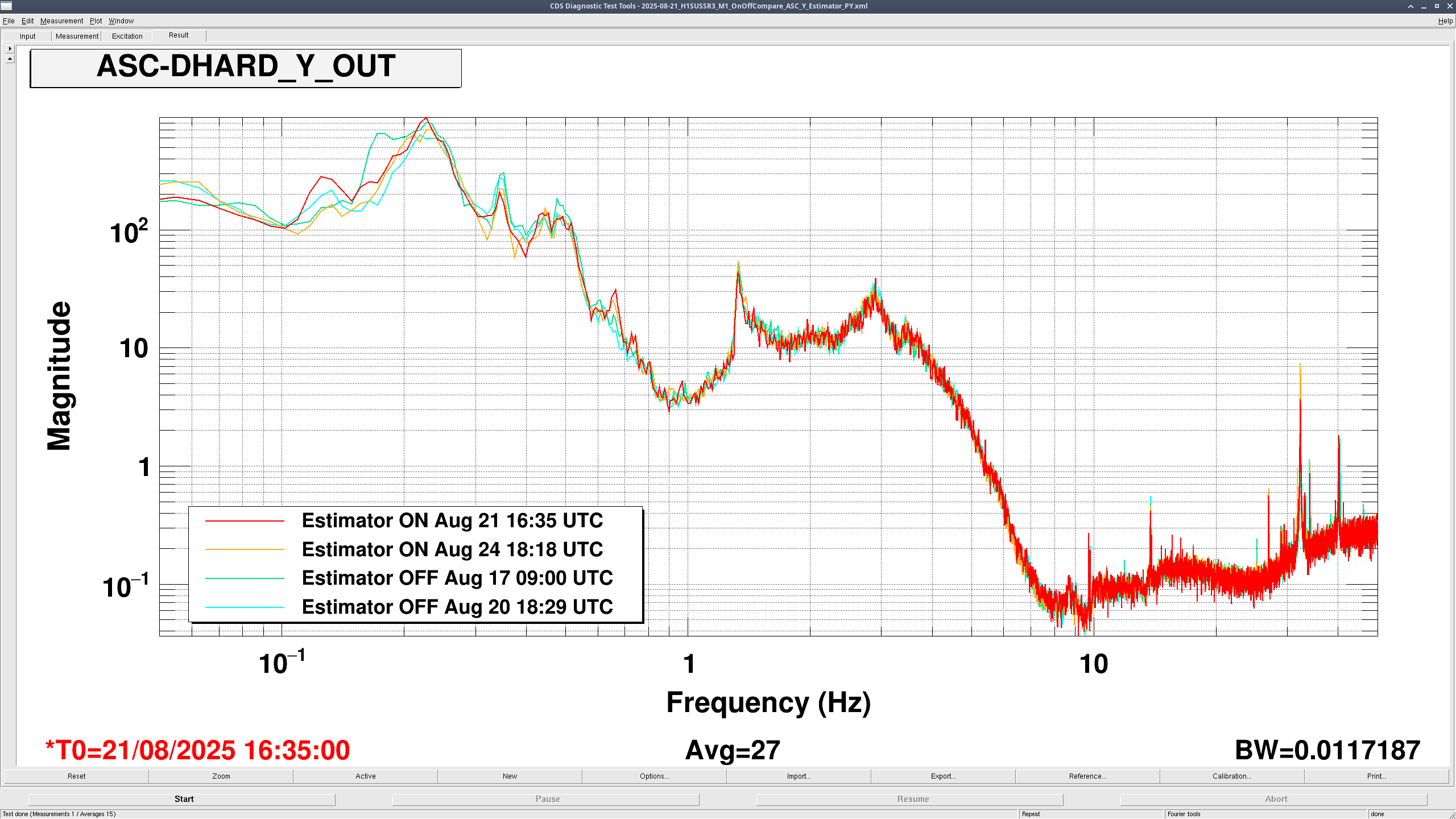
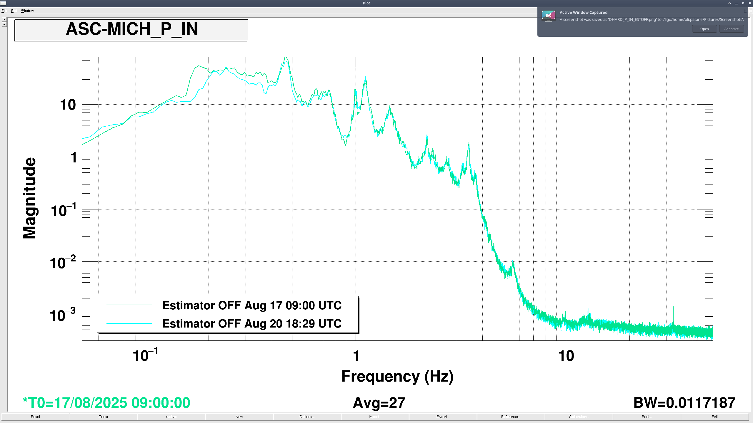
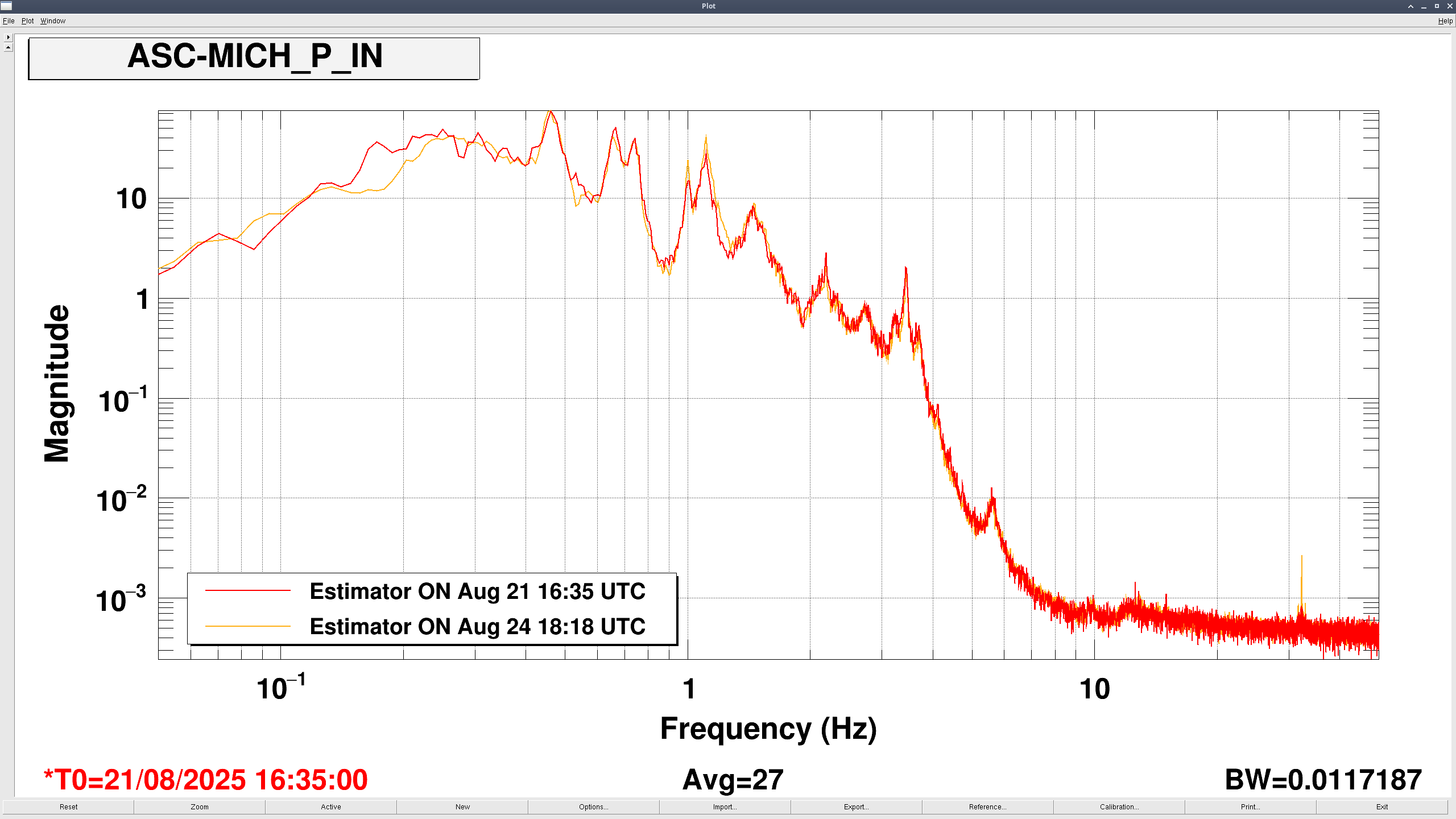
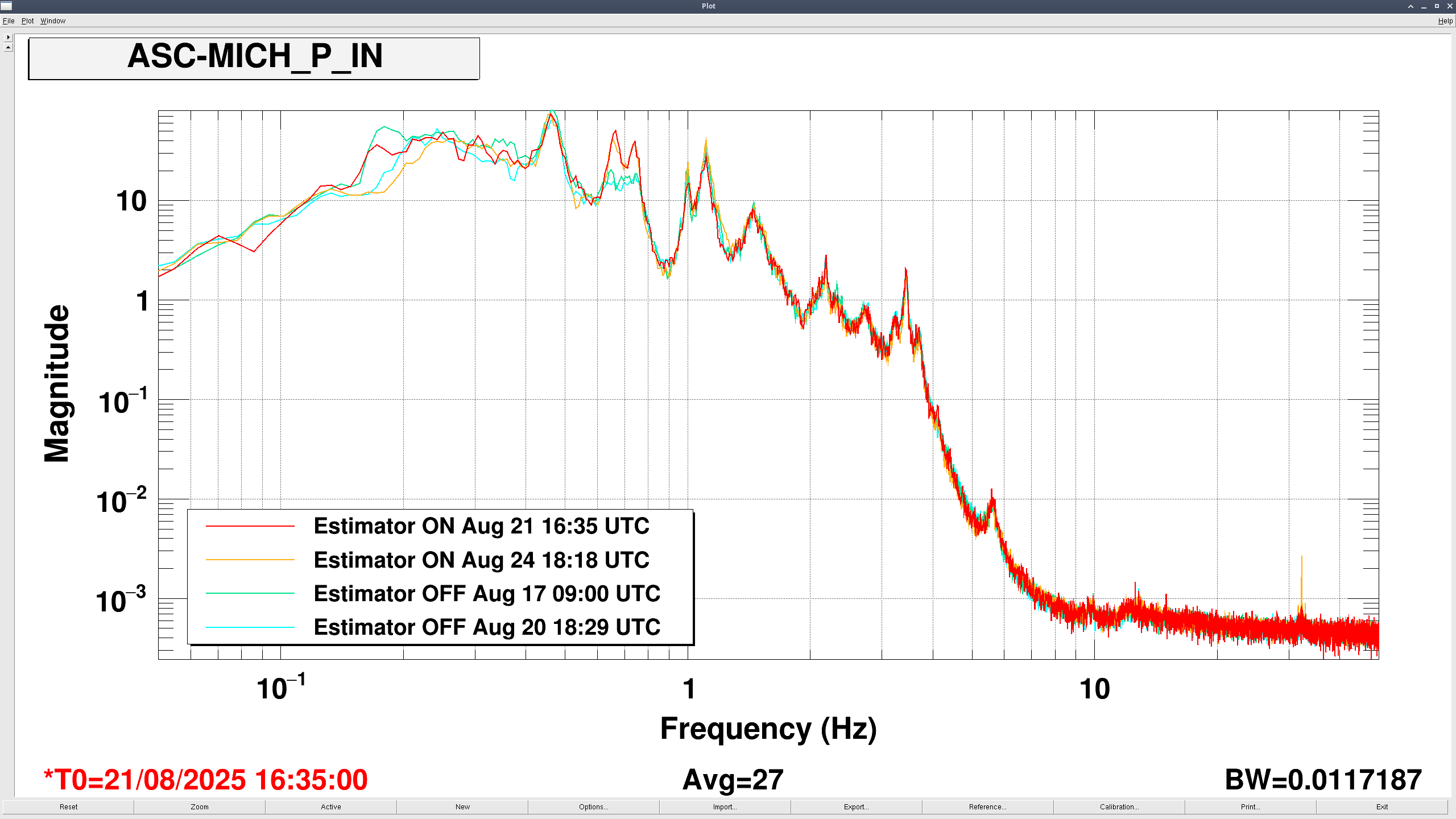
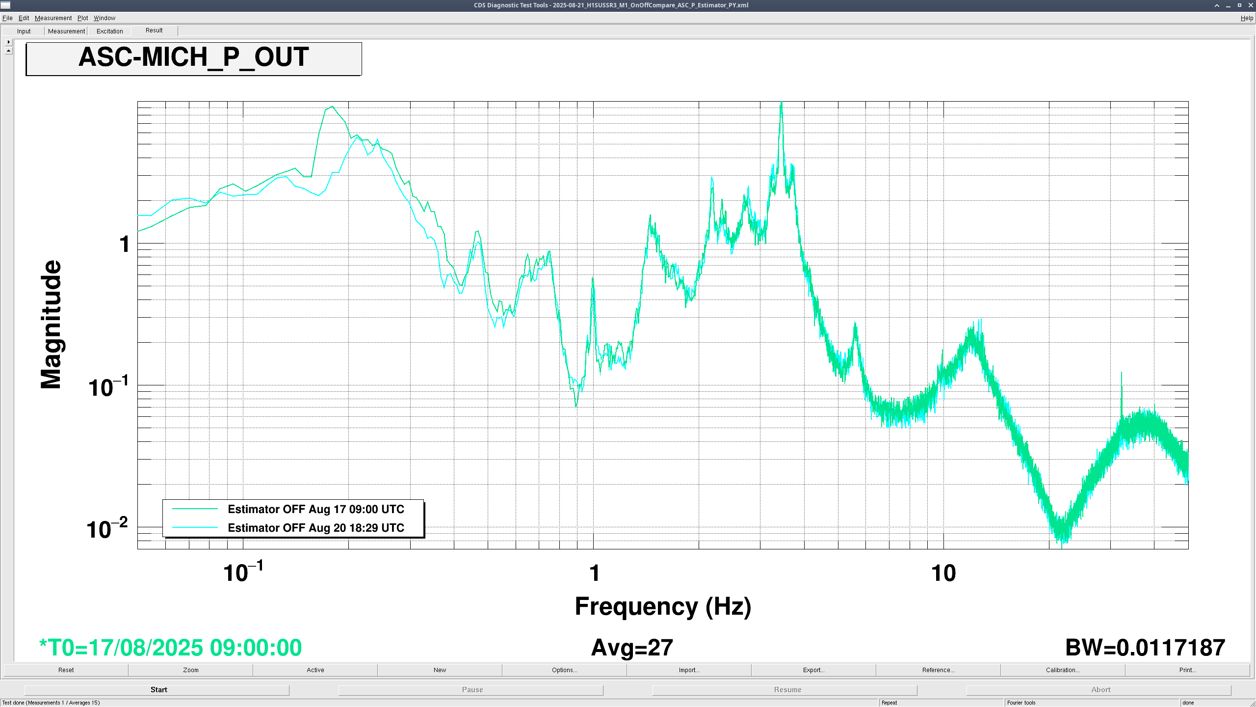
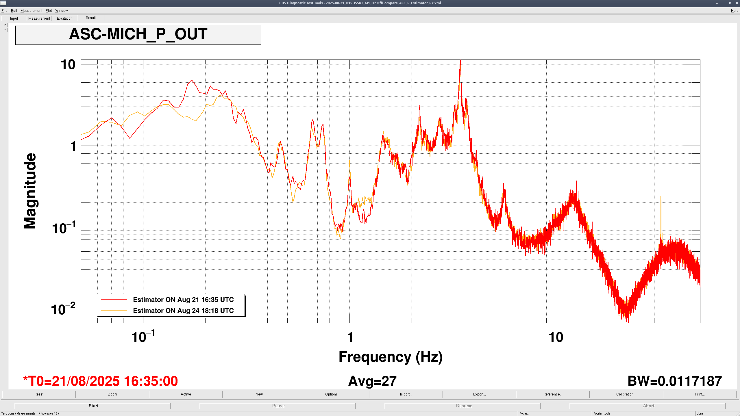
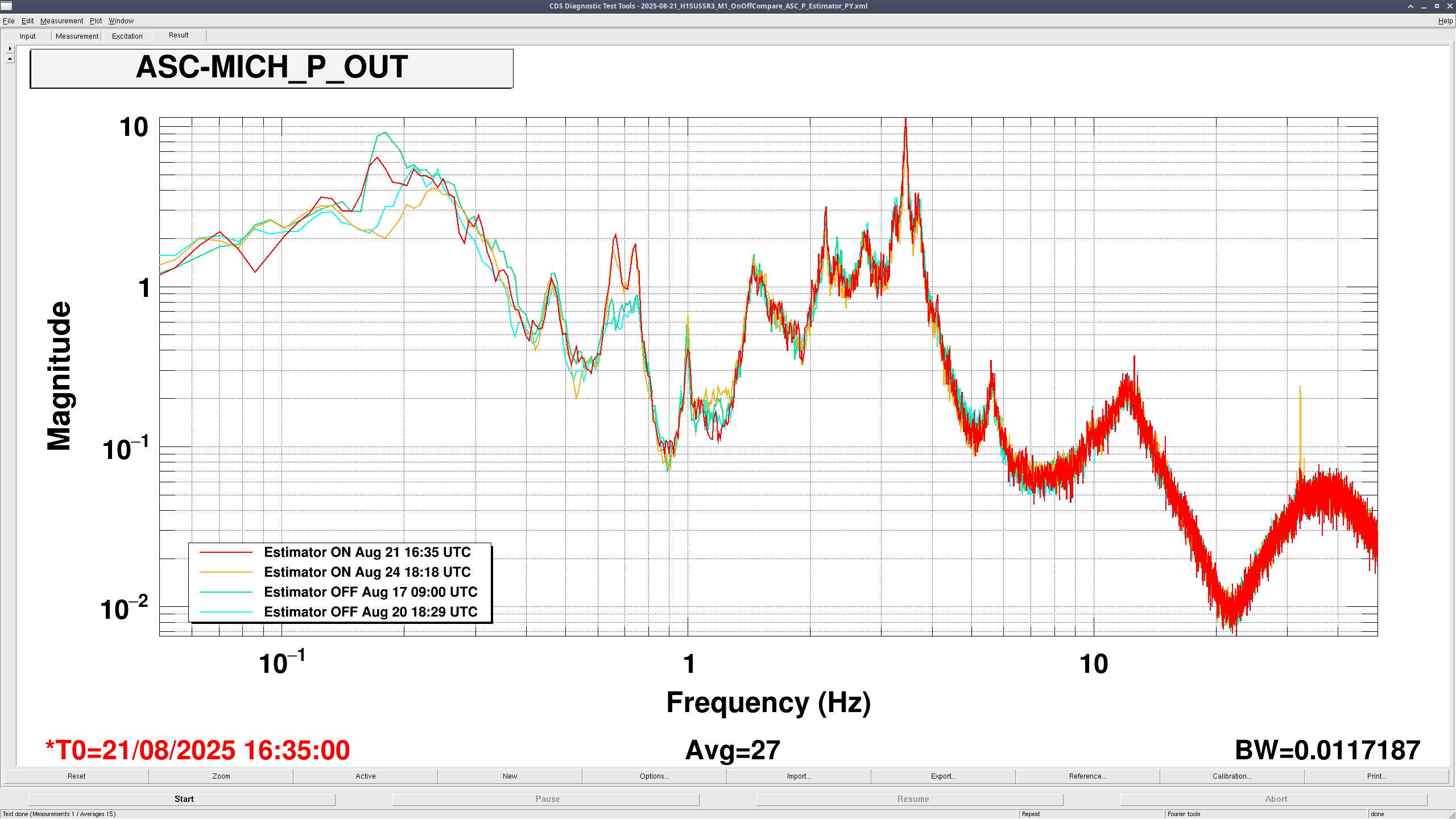
J. Kissel, E. Bonilla

Thanks to the hard and quick work of the Stanford team overnight designing blend filters and super sensor model filters (LHO:86563), I was able to install everything needed to get the H1SUSPR3's estimator up, running, and functional this morning. After having run it for bit during maintenance (and thus corner-station sensor correction was off), I've turned the "use OSEMs or use Estimator" switch to "use OSEMs" such that the SUS is performing in a functionally equivalent way as "no estimator." We'll run like this until (a) I make some plots analyzing the performance and (b) Until Thursday's commissioning period when we're in nominal low noise, so we can do similar ON vs. OFF comparisons with ASC as our metric.

The P and Y estimators were ON from 2025-08-26 18:05 UTC to 19:00 UTC.

Some extra design points beyond whats made in LHO:86563, with the mind-set of "can we 'just' copy and paste SR3's filters into PR3?"
In short: No.
In long:
    The existing OSEM-only damping is different -- all SR3's damping loop's overall EPICs gain is -0.5, where PR3's is -1.0. This is demonstrated by LHO:86554, that means the damped M1 drive to M1 response "damped plant" is different. Namely, on resonance, the loop suppression 1/(1+G), is different because G is different, and thus P/(1+G) is different. This has the effect of shifting the fundamental mode frequencies and changing the residual Q. *That* means two things:
    (1) that the OSEM vs. Estimator blend filters -- which are relatively tight notches around resonances -- in principle, should be different. That being said, depending on the performance we end up getting we could *see* if making the blend filters generically wide enough would work. But, for now, we err on the side of "let's make the blend filters specific" because we have the measurements and the person power.
    (2) The "undamped plant" measurements for the estimator -- which are really "lightly damped" plants with whatever loop suppression is left from the broadband OSEM damping that's still always used; an EPICs gain of -0.1 for SR3 and -0.2 for PR3's damping loop controllers -- are different. So, the filters that are modeling that response -- the Sus. Point drive to M1 response filters and the M1 drive to M1 response filters -- will also necessarily be different. However, the differences are almost entirely resonance shifts and Q changes that are proportional to the differences in 1/(1+G) of the light damping (one with scaled with G = -0.1 and one with G=-0.2). Said differently, so far, only the on-diagonal M1 to M1 transfer functions are proving to be needed, and only the P to P, L to P, and Y to Yaw suspension point to M1 transfer functions are needed, and these are almost identical between PR3 and SR3.

I'll put a comparison of the filters and details of the installation in the comments.


Here're the comparison between the PR3 and SR3 Suspension Point to M1 response transfer functions. These we installed using the scripts /ligo/svncommon/SusSVN/sus/trunk/HLTS/Common/FilterDesign/Estimator/ make_PR3_pitch_model.m rev 12622 make_PR3_yaw_model.m rev 12622 which push the filters from the saved .mat files /ligo/svncommon/SusSVN/sus/trunk/HLTS/Common/FilterDesign/Estimator/ fits_H1PR3_P_2025-08-19.mat rev 12622 fits_H1PR3_Y_2025-08-19.mat rev 12619 (Most are at rev 12622 because the file names had differing arrangements of underscores and hyphens, so I cleaned that up before running.) Notably -- we uncovered the oversight of missing L to P filter install in SR3 (LHO:86567) in enough time to make sure the same oversight didn't happen with PR3. So -- PR3 has - Pitch Estimator P to P, H1:SUS-PR3_M1_EST_P_FUSION_MODL_SUSP_P_2GAP, comparison plot - Pitch Estimator L to P, H1:SUS-PR3_M1_EST_L_FUSION_MODL_SUSP_P_2GAP, comparison plot and - Yaw Estimator Y to Y, H1:SUS-PR3_M1_EST_Y_FUSION_MODL_SUSP_Y_2GAP, comparison plot.Here's the comparison between the M1 to M1 drive transfer functions. These are also installed with the same run of the scripts /ligo/svncommon/SusSVN/sus/trunk/HLTS/Common/FilterDesign/Estimator/ make_PR3_pitch_model.m rev 12622 make_PR3_yaw_model.m rev 12622 which push the filters from the saved .mat files /ligo/svncommon/SusSVN/sus/trunk/HLTS/Common/FilterDesign/Estimator/ fits_H1PR3_P_2025-08-19.mat rev 12622 fits_H1PR3_Y_2025-08-19.mat rev 12619 (Most are at rev 12622 because the file names had differing arrangements of underscores and hyphens, so I cleaned that up before running.)