~10hr lock at 109Mpc in Observing my entire shift so far. Environment calm.
TITLE: 03/31 Day Shift: 15:00-23:00 UTC (08:00-16:00 PST), all times posted in UTC
STATE of H1: Observing at 110Mpc
OUTGOING OPERATOR: Travis
CURRENT ENVIRONMENT:
Wind: 0mph Gusts, 0mph 5min avg
Primary useism: 0.03 μm/s
Secondary useism: 0.12 μm/s
QUICK SUMMARY: Observing, quiet on site.
TITLE: 03/31 Owl Shift: 07:00-15:00 UTC (00:00-08:00 PST), all times posted in UTC
STATE of H1: Observing at 109Mpc
INCOMING OPERATOR: TJ
SHIFT SUMMARY: No issues after EQ rang down and H1 relocked. Observing for the past 5+ hours.
LOG: See previous aLogs.
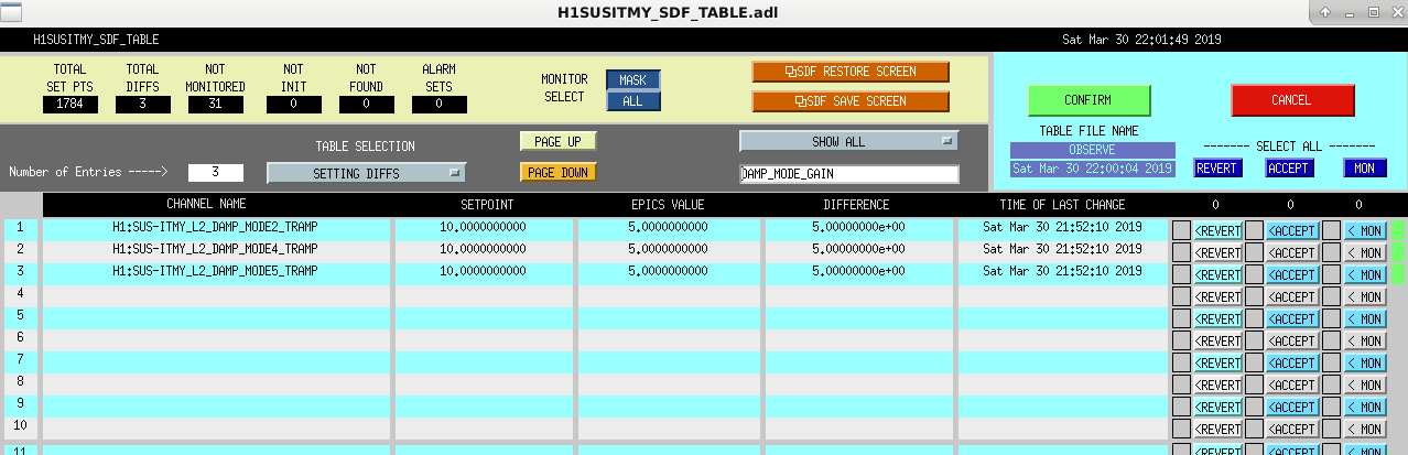
Due to SDF transients:
2019-03-31_11:11:00.150700Z DIAG_SDF [RUN_TESTS.run] USERMSG 0: DIFFS: susitmy: 1
2019-03-31_11:11:55.144777Z DIAG_SDF [RUN_TESTS.run] USERMSG 0: DIFFS: susitmy: 1
H1 locked back up after the EQ rang down with no real issues.
Lockloss while transitioning SEI to LARGE_EQ mode. Two of the ISI Guardians again reported EZCA connection errors, but cleared before I could get a screenshot. Not sure if this contributed to the lockloss or not. I am leaving the IFO in Down until the EQ passes.
Mag 6.2 EQ in Ecuador. Set SEI_CONF to LARGE_ED_NOBRSXY and turned ADS Master Gain to 0.
TITLE: 03/31 Owl Shift: 07:00-15:00 UTC (00:00-08:00 PST), all times posted in UTC
STATE of H1: Observing at 108Mpc
OUTGOING OPERATOR: Jim
CURRENT ENVIRONMENT:
Wind: 4mph Gusts, 3mph 5min avg
Primary useism: 0.07 μm/s
Secondary useism: 0.19 μm/s
QUICK SUMMARY: H1 locked in Observing upon arrival for 2+ hours.
J. Kissel, L. Sun
While Lilli and Joe were tackling signing inside the CAL group's measurement *fitting* scripts, I was slogging away at trying to fight for measuring lower frequency data points to resolve the low-frequency side of the pro-spring detuned sensing function to better constrain the fit.
I was successful in measuring the full features of the detuning, but *answer* for the phase doesn't make sense.
I attach three plots:
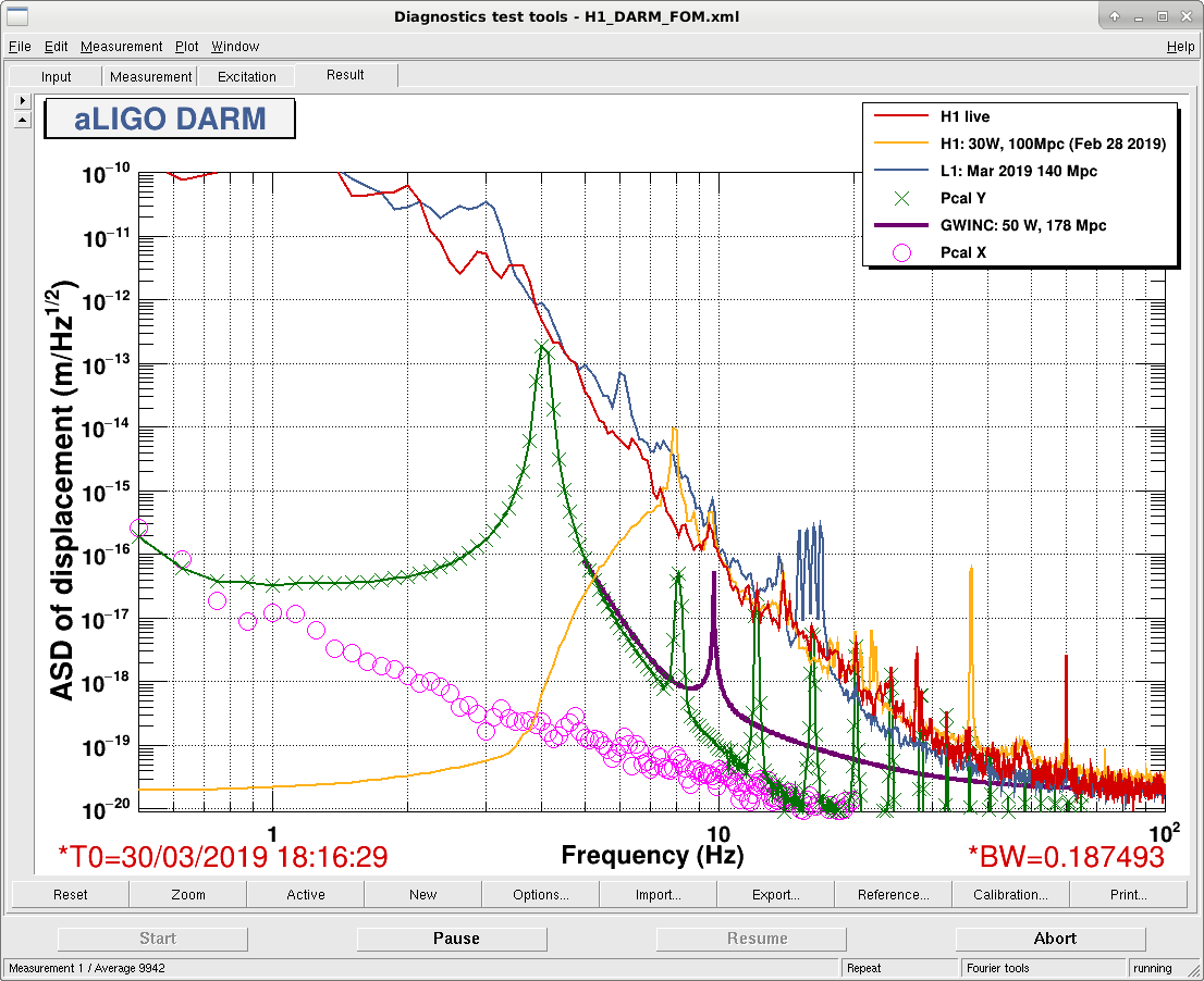
(1) 2019-03-30_H1_DELTAL_EXTERNAL_vs_PCAL_0p5Hzto100Hz.png
We need to drive PCAL at it's maximum in order to get any semblance of SNR / coherence. The ASD of DELTAL external vs. PCAL during the lowest frequency parts of the measurement reveals how many integration cycles I needed in order to get any semblance of SNR [nCycles was 150]. You may notice the RX PD is exposing that the optical follower servo is driving significant amounts of harmonics of power on to the test mass, and be worried that this is spoiling the fidelity of the linear transfer function. Do not fear: we used the PCAL's RX PD as our reference, not the PCAL excitation, so while we may have less power in the fundamental than we request, it is still this power *at* the fundamental that we use as reference in the linear transfer function to DARM.
(2) 2019-03-31_H1_sensingFunction_mcmcModel_vs_measurement.pdf
The output of the MCMC fit on this new data, to show the current status of our canned technology of fitting this data, and
(3) 2019-03-31_H1_sensingFunction_modeldemos_vs_data.pdf
An extension of my demonstrative plot yesterday comparing a pro-, anti- and bogus- spring zpk-decomposable transfer functions, but now includes the physical equation for the detuned sensing function.
None of the models explain the phase of the measured sensing function well.
For the physical model, I dug back in to Evan Hall's thesis P1600295,, gathering material from Sections 2.3, 5.2, and Appendix D, and guided further by his distillation G1601599 plus the Craig / Kiwamu note T1600278.
After a hefty amount of algebra, Evan boils down Equation (3.83) in Rob Ward's thesis, P1000018, whom boiled it down from Eq. (2.20) of Buonanno & Chen (2001) arXiv:gr-qc/0102012, to arrive at his Equation (5.2) that describes the response in terms of poles and zeros,
dP 1 + i f / z
---- = g * ---------------------------------------------------- Eq. (5.2)
dL- [ 1 + i f / ( |p| Q ) - f^2 / |p|^2 ] +/- xi^2 / f^2
where
dP / dL- = the interferometer response (at the AS port) to DARM
g = the optical gain (in this case in [(Watts at AS port) / (meter of differential DARM)])
p = a complex coupled-cavity pole frequency, composed of the arm cavity pole(s) frequency and again, a term related to SRM reflectivity (in amplitude, so sqrt(0.32)) and SRC detuning phase (in radians)
z = a real coupled-cavity zero frequency, composed of the arm cavity pole(s) frequency and a term related to the SRC detuning phase, and this time the readout homodyne angle
Q = the quality factor of the coupled cavity pole frequency, valued determinisitcally by the value of p
xi^2 = the (positive "pro" or negative "anti") square SRC detuned spring pole frequency, depending on lots of things including
- the arm cavity pole(s), laser, and gravitational wave frequencies
- the laser power on the beam splitter,
- the length of the arms,
- the mass of the test masses,
- the SRM reflectivity, and
- the SRC detuning phase
Now -- he discusses in words in the paragraphs following the equation, that this can be boiled down further IF we assume that that SRC detuning phase is set to perfect signal extraction (phi_s = pi/2 = 90 deg) and the readout homodyne angle is also set to zeta = pi/2 = 90 deg. If so, then all the complexity of p and z drops out, p becomes real, and they equal each other, z = p = Re{p},
dP 1 + i f / p
---- = g * -------------------------------------------------- Eq. (K)
dL- [ 1 + i f / ( p Q ) - f^2 / p^2 ] +/- xi^2 / f^2
Note, he says [and I paraphrase] that in this ideal case that "When the SRC detuning phase is 90 deg, then the imaginary part of p is zero, so xi^2 = 0, and everything collapses to a single pole equation, 1 / (1 + i f / p)." But it's too late, and I don't grok that yet.
So, I assume that Craig and Kiwamu's "small detuning" means that the above Eq. (K) is in play, so I plot this physical response against
- the pro- and anti- approximations that we're able to create in Foton for both positive and negative values for xi^2,
- the bogus spring we mistakenly modeled two days ago, and
- the data.
None of these models agree with the data, because the data's phase implies right-half-plane, complex poles.
I need to sleep on this...
I also attach the data for any of you bold enough to try to model this data while I sleep.
[ freq linearmagnitude linearmaguncertainty phase(deg) phase(deg)uncertainty]
rawData = load(dataFile);
tf_freq = rawData(:,1);
tf_mag = rawData(:,2);
tf_magunc = rawData(:,3);
tf_pha = rawData(:,4);
tf_phaunc = rawData(:,5);
errorbar(tf_freq,tf_mag,tf_magunc,'k*')
errorbar(tf_freq,tf_pha,tf_phaunc,'k*')
Also, for the record -- we've changed NOTHING in the CAL-CS front-end pipeline, so you should expect the PCAL 2 DELTAL systematic error to be the same yesterday -- at the +/-1% above 20 Hz.
The actuator is still at 0.95 of what was expect it to be, but we at least now understand that it's this poor understanding and/or ability to create a real-time filter to compensate the sensing function that causes the error.
Any sudden gains in range you saw in the BNS range were because we were turning off all intentional lines -- namely calibration lines (at 30 Hz) and TCS tracking lines (at 65 Hz) -- which eat up a few Mpc.
You can still trust the calibration as stated.
After relocked accepted the ITM-Y SDF Diffs.
Jeff K. & Lili S. finished their calibration measurements. Have been in Observing for the past 2 hours. The IFO is currently locked at NLN, with a range of 109.1Mpc. Environmental conditions remain favorable. There are no significant issues or difficulties to report.
Jeff K, Joe B, Lilli S,
We have fixed a few problems in sensing.py for the pro-spring fitting.
1) Jeff has fixed the pro-spring TF calculation yesterday (see 48057). There's still one imaginary "j" missing in the line below:
Line 740: est_opt_response_tf = mu[0] / (1.0 + 1j*xdata/mu[1]) * (xdata**2/(xdata**2 - mu[2]**2 + 1j*xdata*mu[2]*mu[3])) * np.exp( -2.0*np.pi*1j * mu[4]*1.0e-6 * xdata )
2) The signs were wrong when calculating the detune TF.
Line 65: detuneFunction = signal.TransferFunction([1,0,0],[1,-2.0*np.pi*abs(detuneSpringFreq)/detuneSpringQ,(2.0*np.pi*abs(detuneSpringFreq))**2])
After these two fixes, the pro-spring fitting is much better than before (good enough above 20Hz). See the "before fix" and "after fix" attachments.
3) The priors of fcc, fs, Q are not close to the true values. As a result, the MCMC will draw samples far away from the MAP values. The corner plots include a lot small "islands", although the MAP values returned are valid (see the attached "beforeChangePriors" plot). This would impact the samples used for calculating uncertainty budget in the future. We have adjusted the priors to be closer to the true values. A better fix remains to be done to read in the priors instead of hard coding them.
4) We have calculated and output the "Inverse Sensing FOTON values" and "Inverse Sensing without cavity pole FOTON values for CFTD path" for the pro-spring case. --> Take s^2/(s^2 - s0^2 + i*s*s0/Q) and solve denominator for zeros, i.e., the two zeros are the two conjugate complex roots.
cf. for anti-spring --> Take s^2/(s^2 + s0^2 - i*s*s0/Q) and solve denominator for zeros, and the two zeros are real.
We are taking more measurements including low frequencies to verify the fitting. A new model needs to be created and installed.
IFO is actually locked at NLN_CAL_MEAS.
TITLE: 03/30 Day Shift: 15:00-23:00 UTC (08:00-16:00 PST), all times posted in UTC
STATE of H1: Calibration
INCOMING OPERATOR: Jeff
SHIFT SUMMARY: Lost a ~50hr lock, did an initial alignment and came right back up. CAL measurements going on currently.
LOG:
1821 Out of Observing for Cal measurement
2017 Lock loss
2030 Dave B restart h1edc
2054 Initial alignment
2208 Observing
2247 Out of observing for CAL meas.
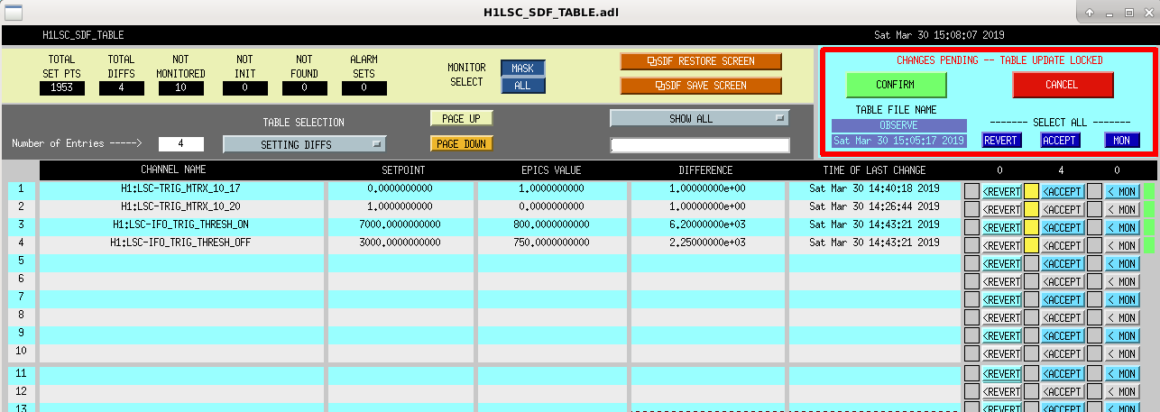
Had to do initial alignment, couldn't get good power with POP18 in DRMI (~50 max). CAL CS SDF diff from tiny changes, I just accepted these. LSC SDF diffs that I didn't know about, so those are attached.
2019_03_30 13:31 h1edc
This alog has been edited.
I think that we have understood one of reason that we have had trouble with the stability of our DARM loop over the last few months, which I've tried to explain in a dcc note: T1900148. The summary is that we are using length to angle decoupling, and because our spot positions are far off center we also are using gains of about 5 in the angle to length decoupling on the ETX PUM (a DARM actuator) to avoid having the angular drive show up in length. Since the output of the length to angle decoupling doesn't go through the angle to length decoupling filter, the output of that filter couples to DARM through the spot mis centering, which has been large enough to cause instabilities and calibration problems.
There have been several problems with the stability of the DARM loop over the last few months that might be explained by this, including the 4.2 Hz instability, which was initially solved by adding a boost to the PUM lock filter (47164) but has come back in the last few weeks, There have also been several attempts to change the DARM loop in ways that should have been stable according to the model but weren't, this effect is probably contributing to that difficulty.
This morning Niko and Jenne have been struggling with 4.2 Hz locklosses again, so we took a guess that turning off the L2P and L2Y might help fix the problems at 4.2 Hz, and that turning off the boost in the PUM stage would give us more phase margin for the crossover around 8 Hz and might help us avoid the locklosses we've had with the L2A off. So far it seems that this is working. If we can run like this it would make the calibration more accurate and make understanding our DARM loop easier.
The two most obvious ways to get rid of this parallel DARM actuation path are to set the A2L gains to zero, and turning off the L2A decoupling. We don't want to set the A2L gains to zero because we do not want the spot to be centered on the optic (power recycling gain, point absorbers). We would expect that turning off the L2A decoupling will increase the size of the ASC control signals. We have never had accurate measurements for the length to angle decoupling above 2.5 Hz, these filters are rolled off at around 10 Hz.
Some other conclusions from thinking about these cross couplings more: (updated)
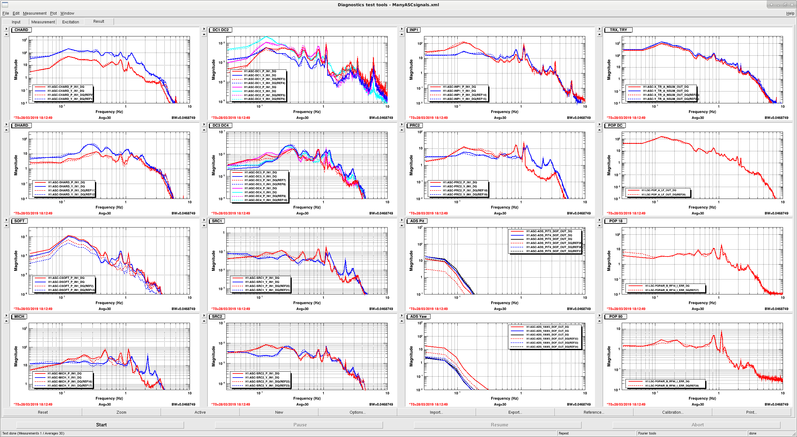
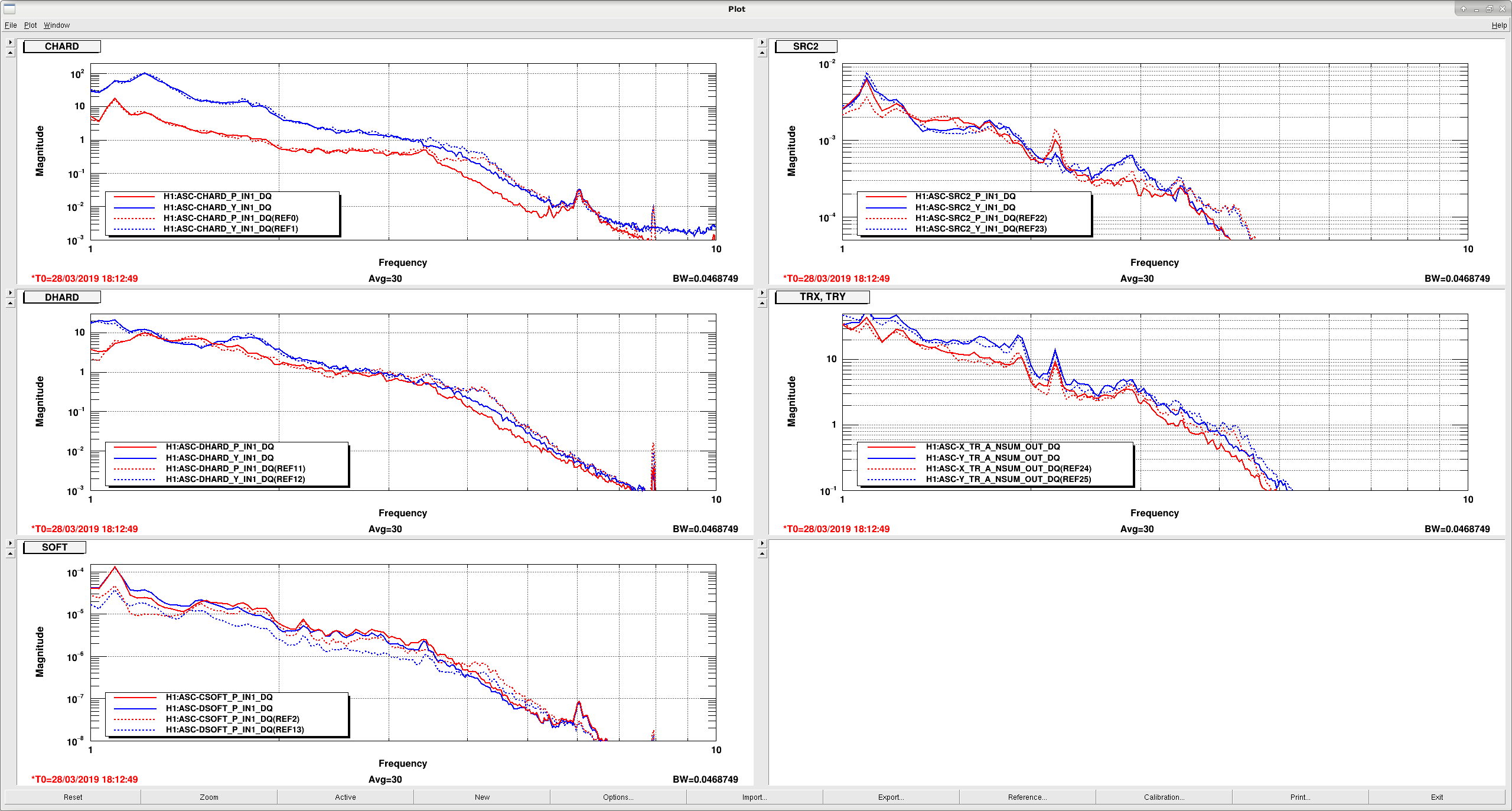
In the attached figures (one with many signals, the other zoomed in on the signals that have a relevant change) show a reference time (dashed traces) from last night, when we did have our previously-nominal L2A filters and the PUM boost on versus our current lock without the L2A or PUM boost. You can see that all of the arm degrees of freedom (CHARD, DHARD, CSOFT, DSOFT and ADS) see much less motion at ~4 Hz, but the SOFT degrees of freedom see more motion at lower frequencies. This isn't too surprising since the L2A filters were measured with good coherence up to about 2 Hz, but not above there. On an upcoming Tuesday when we have time, we'd like to take data to get these L2A filters better coherence (JeffK started this Tuesday, but it's really hard to get good coherence).
Relocked this evening with no apparent problems. Guardian setup the ETM-X L2_LOCK_FILTER as described in Sheila's E-Mail to the operators. The Qprime (FM7) was turned on and the FM5 boost4.5 was turned off. The gain for L2_L was set to 23.00. The L2_L current state is 0x6030004, the correct state is 0x6000004, and the state is flagged as bad.
ETMX violin mode 9 is increasing slowly because the gain was turned off by the violin damping guardian. This is a usual situation as of late, but it means that I will need to go out of observing soon to add damping. I'll to wait for single IFO time.