h1susey has crashed. Similar to h1lsc0 this morning it looks like the models are still running and the suspensions are still being damped. We have lost DAQ data from this machine and EPICS monitoring/controls.
If we need to restart this system, please call me on my cell phone and I can do this remotely.
h1susey crashed at 19:00 PDT (02:00 Sun 7th UTC).
current status of SUS-EY.
I spoke with Richard on the phone last night soon after the crash and we agreed we could leave this system overnight because both the software-watchdog (running on h1iopsusey) and the independent hardware-watchdogs were functioning.
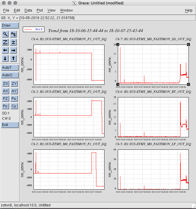
I realized we can indirectly monitor what the h1susetmy model is doing by looking at the coil current monitors being acquired by the h1susauxey model. Attached plots show 24 hours of M0_F1 IMON against h1susetmy_cpu_meter, 7 days of M0_F1_IMON, and 24 hours of all the ETMY M0 IMONs.
It looks like the suspension has changed state around 4am this morning.
Would the first commissioner on site today please call me on my cell phone and we can schedule a restart of h1susey.
You have to be careful leaving the front end in this state, at least when it come to guardian. If a guardian node can't see EPICS channels it needs it goes into a CERROR state, in which it won't progress on it's graph until the needed channels are recovered.
We had a very similar failure at LLO last week, while the IFO was at full lock. The IFO kept operating otherwise normally, but the ISC_LOCK node went into CERROR. When there was a lockloss the node was still stuck and the DOWN state was not executed. This can be bad since certain resets don't take place in a timely manner, which can cause things like violin modes to et rung up.
Looks like that's exactly what happened here. See alog 44384 for a few notes.
Continuing the activity described in 44366, I measured the response of REFL WFS in yaw to CHARD, INP1, PRC1 and PRC2. Here's the sensing matrix, measured with a line at 8.5 Hz (CHARD ampl. 1.0, INP1 ampl. 1e6, PRC1 ampl. 0.01, PRC2 ampl. 0.3). The units are REFL_WFS units / ASC filter bank output. Therefore a direct comparison of the different degrees of freedom is difficult, since the actuator response is different in all cases (I can't see the excitation in the OPLEV signals, so I don't have a calibrated motion sensor).
| CHARD | INP1 | PRC1 | PRC2 | |
|---|---|---|---|---|
| REFL_A_RF9 | -0.000529 | 0.0553 | 0.0228 | 0.202 |
| REFL_B_RF9 | -0.000591 | 0.0278 | 0.0511 | 0.246 |
| REFL_A_RF45 | -0.000441 | 0.0686 | 0.0123 | 0.248 |
| REFL_B_RF45 | -0.000484 | 0.0461 | 0.0160 | 0.276 |
If we use this matrix and the ASC yaw input matrix currently in use for CHARD and INP1, we get the following response
| CHARD | INP1 | PRC1 | PRC2 | |
|---|---|---|---|---|
| CHARD err | -1.2764e-03 | 1.2079e-01 | 5.3820e-02 | 6.1000e-01 |
| INP1 err | -1.9580e-04 | 3.4960e-02 | -8.4000e-04 | 4.8400e-02 |
| REFL_A_RF9 | REFL_B_RF9 | REFL_A_RF45 | REFL_B_RF45 | |
|---|---|---|---|---|
| CHARD | 11.38 | -4.048 | -11.011 | 5.170 |
| INP1 | -0.178 | 0.138 | 1.495 | -1.336 |
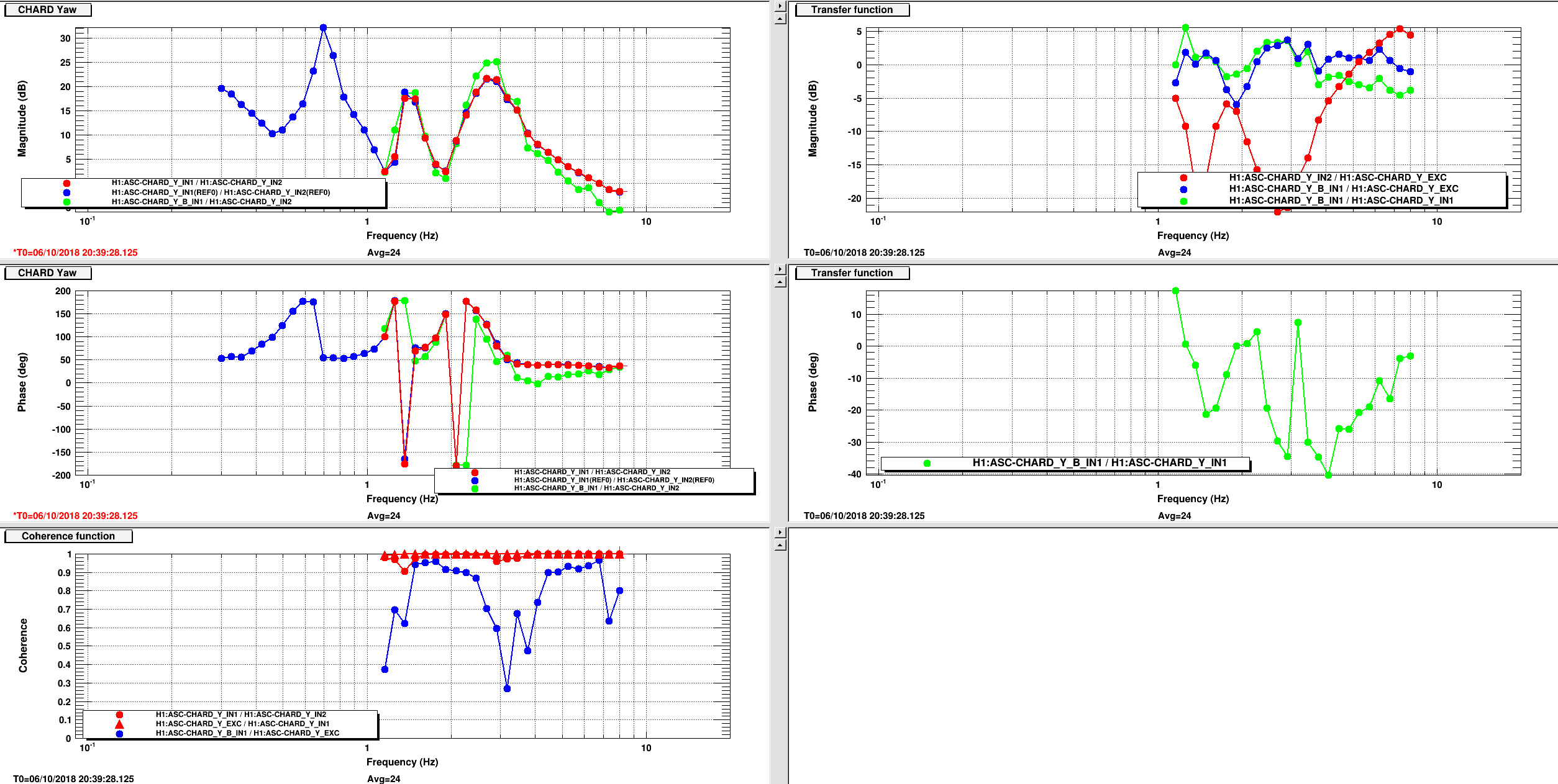
This is quite different from the sensing matrix currently in use. I plugged those numbers into the CHARD_Y_B row of th input matrix, and measured the response to a CHARD sweep. If the new combination and the old one were equally sensitive, one would expect that CHARD_Y_B_IN1 / CHARD_Y_IN2 = CHARD_Y_IN1 / CHARD_Y_IN2 and that CHARD_Y_B_IN1 / CHARD_Y_IN1 = 1. This is not the case... Actually the new combination shows even less phase margin than the old combination. So the CHARD_Y sensing mystery deepens.
I left the IFO locked in DC_READOUT, with a CHARD_Y sweep sine going, measuring the coupling to all other yaw loops.
h1lsc0 general core looks like it has crashed. The models continue to run. No IPC problems on receiving models, no DAQ problems outside of h1lsc0.
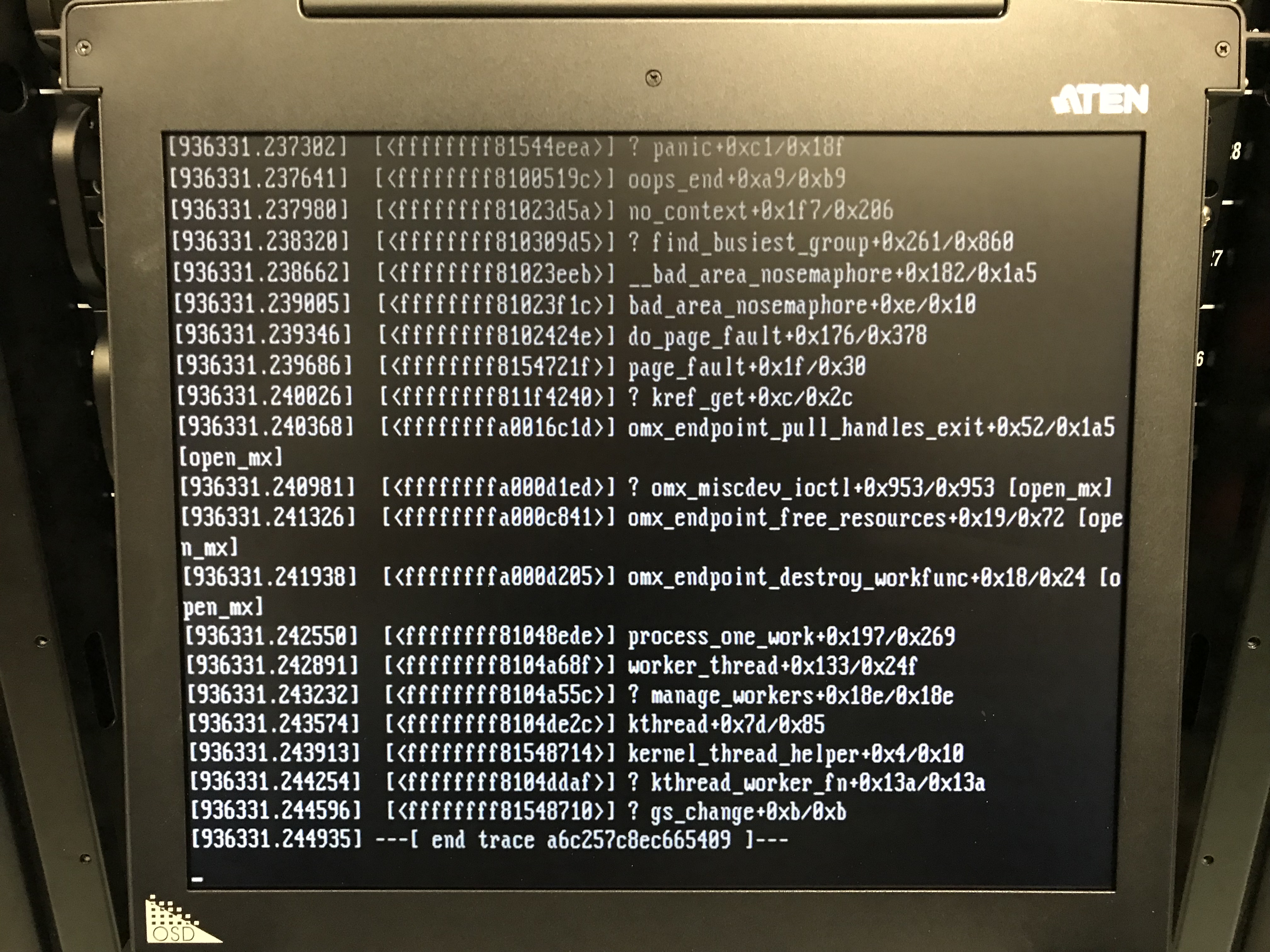
Gabrielle is on site and is taking a picture of h1lsc0's console before we start the recovery process.
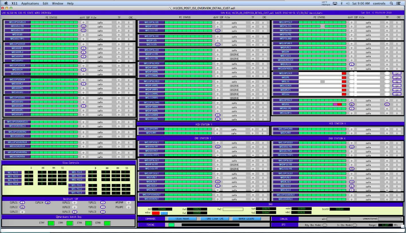
Here is the CDS overview:
Screenshot from the H1LSC0 terminal
Console was unresponsive. I remotely disabled h1lsc0's Dolphin switch port and Gabrielle pressed the RESET button on the front panel.
Restart went well, h1lsc0 is back.
Trending the CPU usage of H1LSC0 and one of the EPICS channels, it looks like the crash happened around Oct 06 2018 12:56:58 UTC. This should be 6am local time
The IFO is locked at a state that looks like PREP_DC_READOUT_TRANSITION, but:
I can't find any instruction on how to fix this in the wiki...
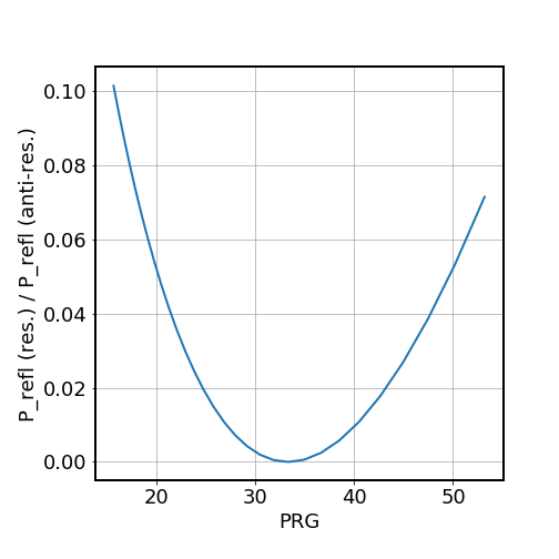
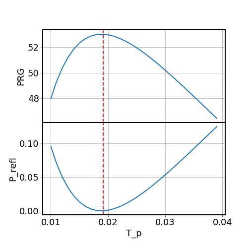
In the attached plot we show the refl pd power as a function of power recycling gain (PRG). Here the x-axis is the PRG, the y-axis is the refl PD power, normalized by the power when the carrier is anti-resonant in CARM & PRC. In generating the plot we vary the arm losses as a parameter to compute the PRG and refl power simultaneously.
Daniel suggested that in the future we might consider changing the PRM transmissivity to optimize the power recycling gain (PRG), given that we have less losses in the arms.
In the attached figure we show the PRG and reflected power P_refl (normalized by the anti res value) as a function of the PRM transmissivity. In the calculation we have assumed a total loss in one arm is 67 ppm (55 ppm loss at the ITM, 8 ppm scattering loss at the ETM, and 4 ppm transmissivity of the ETM), which gives a PRG of 50 for the current PRM transmissivity of 0.03. The red-dashed line shows the theoretically expected optimal T_prm that maximizes the recycling gain, and can be calculated based on the simple relation (cf. eq. 2.18 of Evan Hall's thesis, assuming T_itm=0.014):
T_prm (optimal) = 4 eta_arm / T_itm = 1.91% * (eta_arm / 67 ppm),
where eta_arm is the total loss per arm. This leads to an optimal recycling gain of
PRG (optimal) = T_itm / (4 * eta_arm) = 52.2 * (67 ppm / eta_arm).
Georgia, TVo
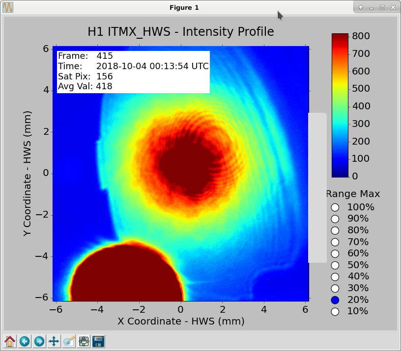
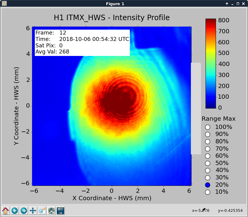
We walked the picomotors on the periscope for ITMX HWS in order to get rid of the prompt reflection and reduce the clipping on the baffles. Attached are the before and after photos.
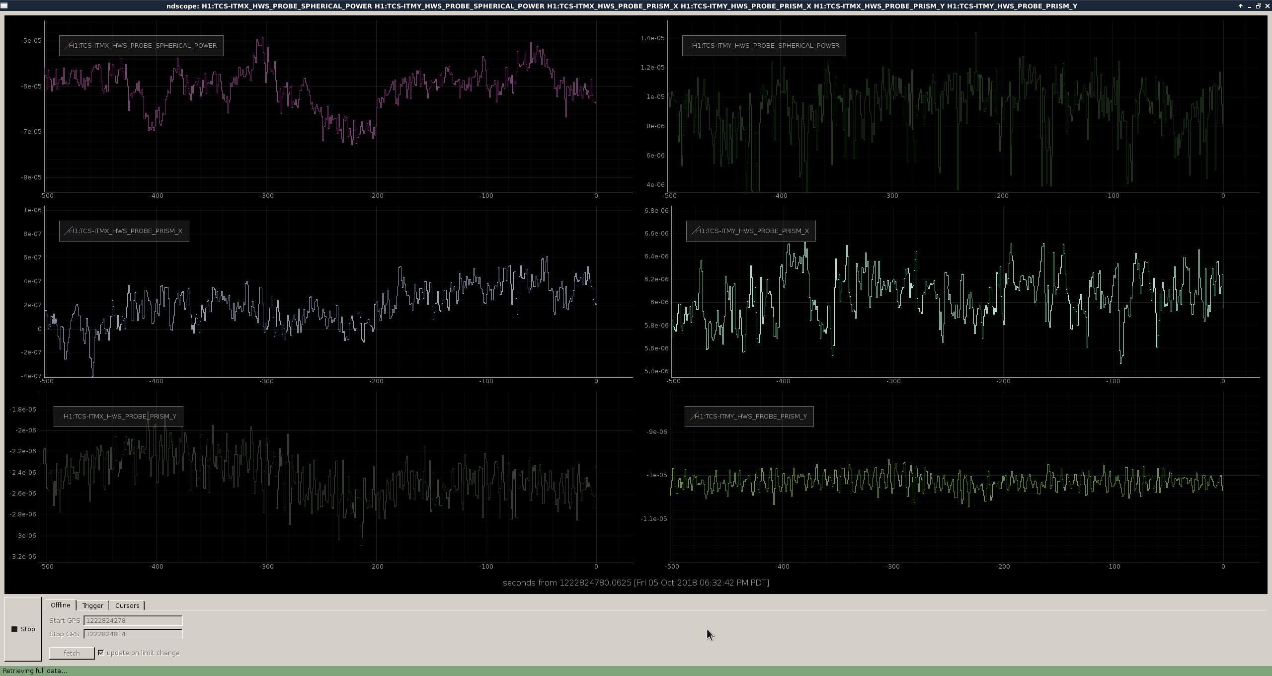
During about 30 minutes of DC Readout when no transient heating is being applied so we expect very small changes in spherical power as a function of time, the ITMX HWS is still noisier than ITMY HWS by about a factor of 3 just looking at the time series. This is better than before when we had a prompt reflection that was screwing up the fitting for the spherical power, maybe we can go back to the same alignment but digitally subtract the beam and keep the useful HWS beam, this is in progress.
After this alignment adjustment the noise got better but attached are the gradient plots for about 5 minutes for both HWS, it show that ITMY sees much less optical path distortion than ITMX and there seems to be a very large gradient vector for ITMX around coordinates=[+0.01, +0.05]. At first glance, this may be dust somewhere in the optical path so we'll investigate the optical table with an ion gun. This "dot" remains persistent for multiple time frames and was present both before and after the pico-ing
There is also a large amount of contours in the upper left hand section, which looks like it's due to the single gradient arrow at coordinates=[-0.1,+0.75]. It is not obvious the root cause since it doesn't look like a normal fringe pattern and we only have one real data point there but we can try to pico away from the left hand side of the baffle and see if this improves the contour plots.
Jeff K., Evan G. Summary: We've reprocessed the measurement transfer function sweeps taken yesterday, and have found the coupled cavity pole was measured to be 429 Hz +/- 6 Hz, quite consistent with computing the pole from the arm reflectivities reported in galaxy (and use Eq 12 from T1500325) -- 433 Hz. We've since identified that Craig's single pole MCMC model (see LHO aLOG 44351) did not include detuned spring, and had a flaw in its log likelihood function resulting in an incorrect fit. The other physical parameters are fit with this process as well and described in the details below. Details: We used the new pyDARM infrastructure that has been developed over the last several months to analyze the transfer function sweeps taken yesterday evening. These measurements were quick 'n dirty; leading into and during an observing run, we would have more careful measurements to reduce any uncertainty. So we expect some reduction in uncertainty in future measurements. pyDARM can perform MCMC fitting to the physical parameters of the coupled cavity optical response. The results of that fit are listed below: Optical Gain K_C [ct/m] 3.552e6 +/- 3e4 Couple Cav. Pole Freq. f_c [Hz] 429 +/- 6 Residual Sensing Delay tau_C [us] 2.75 +/-1.7 SRC Detuning Spring Freq. f_s [Hz] 5.815 +6/-4 Spring Qual. Factor Q_s [ ] 4.2 +/- 6.5 A Gaussian process regression was used to establish potential unknown systematic errors, but this is merely for practice. We know - This was a quick 'n dirty measurement with poor uncertainty and limited frequency range, and - This is only one measurement, and we really want several to many measurements to nail down real unknown systematics Here's the resulting design string we have put into Foton and loaded into the CAL-CS model (in the H1:CAL-CS_DARM_ERR filter bank) to improve on what was installed yesterday SRCD2N (as "O3_D2N" in FM9): zpk([428.9869;5.1756;-6.5327],[0.1;0.1;7000],1,"n")gain(3380.64) Gain (as "O3Gain" in FM10): gain(2.815e-07) We fit these results with the following code: /ligo/svncommon/CalSVN/aligocalibration/trunk/Runs/O3/H1/Scripts/process_sensingmeas_20181004.py
I injected a line at 8.5 Hz in both CHARD yaw (amplitude 1.0) and INP1 yaw (amplitude 3e6) and measured the response of the REFL WFS (in units of WFS / loop output)
| CHARD YAW | INP1 YAW | |
|---|---|---|
| REFL_A_RF9_I | -0.00265 | 0.227 |
| REFL_B_RF9_I | -0.00296 | 0.113 |
| REFL_A_RF45_I | -0.00240 | 0.351 |
| REFL_B_RF45_I | -0.00272 | 0.237 |
The RF9 signals have a slightly better SNR than the RF45 signals, so I inverted the 2x2 RF9 matrix (and rescaled so that the response should be the same as the input matrix in guardian)
| REFL_A_RF9 | REFL_B_RF9 | |
|---|---|---|
| CHARD | -1.50 | 3.68 |
| INP1 | 1.00 | -0.88 |
For comparison, now we are using the following input matrix:
| REFL_A_RF9 | REFL_B_RF9 | REFL_B_RF45 | |
| CHARD | 1.00 | 0.20 | 1.30 |
| INP1 | 1.00 | -0.40 | -0.20 |
This matrix has the same response as the new ones for the diagonal CHARD > CHARD and INP1 > INP1 elements, but the off diagonal element from INP1 to CHARD is much larger.
Finally, to have a complete picture we should measure the PRC1 and PRC2 response in the REFL WFS.
I've updated the HWS code so that the gradient field data is saved as HDF5 files instead of PICKLE files. I also updated the wavefront viewing utility so that it correctly extracts data from the new HDF5 files. I tested this at CIT on the HWS system and it worked pretty seemlessly.
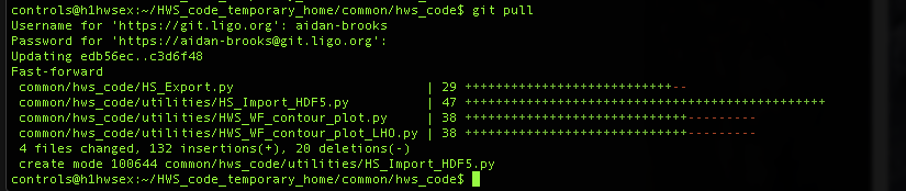
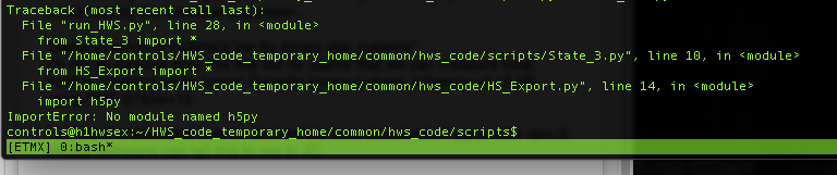
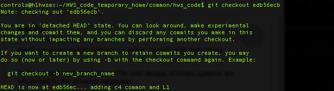
Per work-permit 7857, I pulled the latest version of the code from the GIT repo on H1HWSEX and tried running it on that machine. It didn’t work because the H5PY package isn’t installed. I didn't have time to fix this issue so I reverted the version of the code to the earlier (working) version on GIT and restarted the HWS code.
Updating files:

Failure during execution:

Restoring earlier version of HWS_code

I created an improved script to analyze the Optical Spectrum Analyzer data [the script can be found in /opt/rtcds/userapps/release/isc/h1/scripts/osa.py]
In summary:
gabriele.vajente@zotws2:~/$ /opt/rtcds/userapps/release/isc/h1/scripts/osa.py -h
usage: osa.py [-h] [-f FILENAME] [-t TIME] [-o OUTPUT] [-r REPROCESS]
optional arguments:
-h, --help show this help message and exit
-f FILENAME, --filename FILENAME
File where the time series of sideband and carrier
powers will be saved
-t TIME, --time TIME Duration of plotting window in seconds
-o OUTPUT, --output OUTPUT
Name of a folder where the average OSA scans will be
saved
-r REPROCESS, --reprocess REPROCESS
Reprocess scans from a folder, and save a
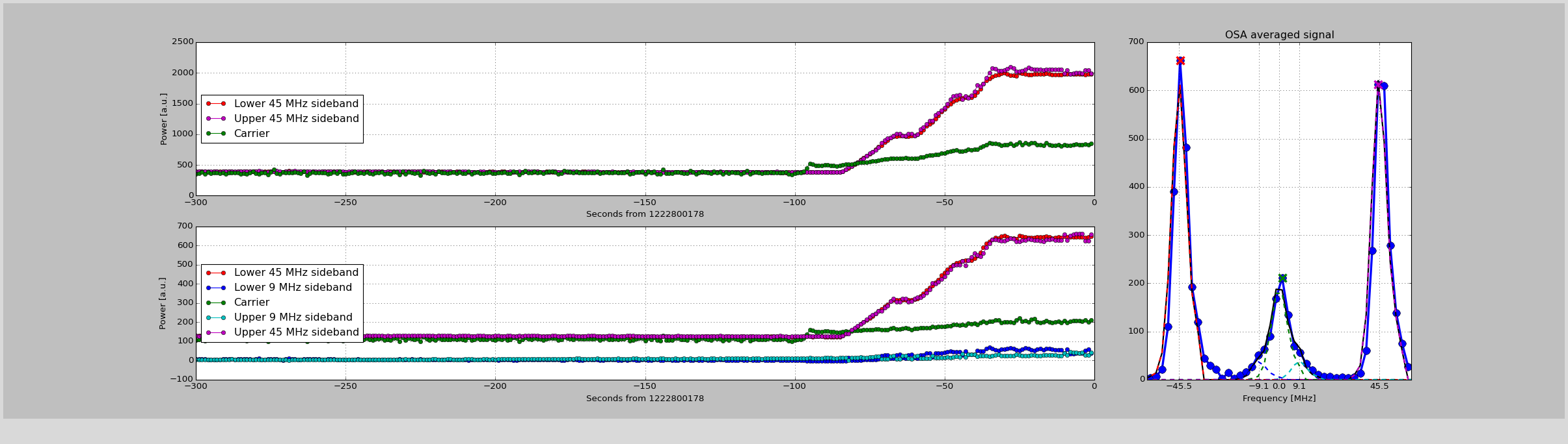
reprocessed.txt file in thereWhen running online, the script produces a plot like the one below, taken during a power up.
The two left panels contains the time traces of the peak powers. The top panel shows the "simple" peak reconstruction as explained above (simply identify the 45MHz peaks, integrate their power, find the largest peak in the middle and integrate its power). The bottom panel instead shows the more "advanced" reconstruction of the 45 MHz, 9 MHz and carrier peaks, by fitting peaks at the correct frequencies.
The right panel shows the latest averaged scan (blue dots and trace) plus some fitting and peak identification traces: the red, green and magenta X show the peaks used for the "simple" reconstruction (time traces in the top left panel); the dashed curves show the individual fits to the sidebands and carrier peaks (time traces in the bottom left panel); the black trace shows the sum of all fitted sideband and carrier peaks.
The 9MHz sidebands are very close to the carrier peak. When at low power, it's hard to resolve them. Even at 10W, they barely make bumps on the side of the carrier peak. So their power measurement has a quite large uncertainty and should be taken with care.
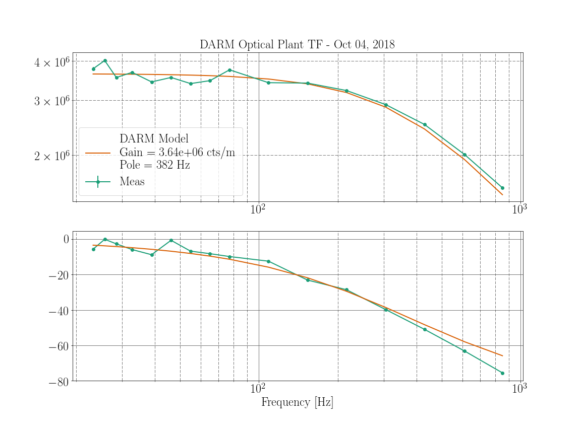
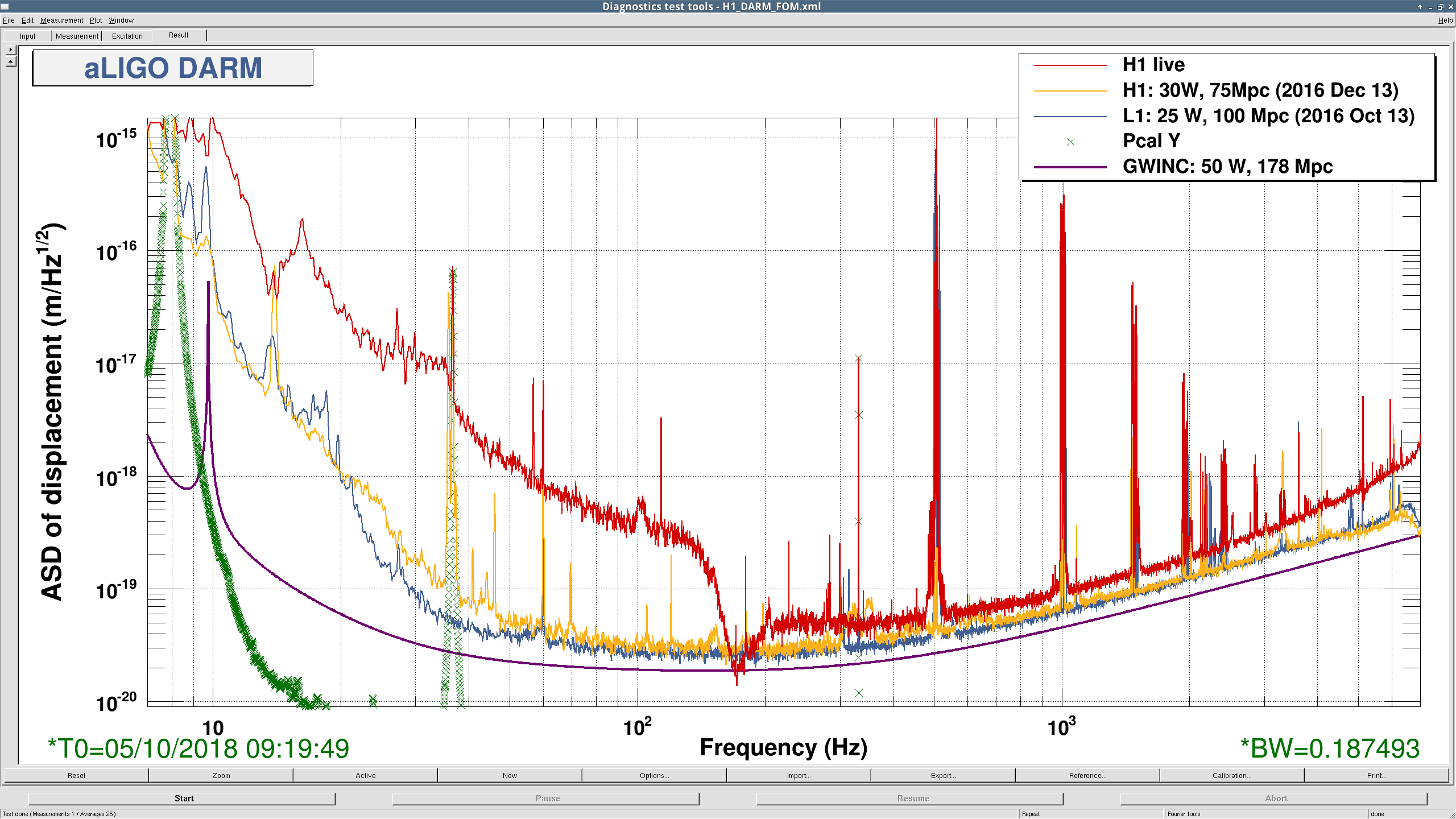
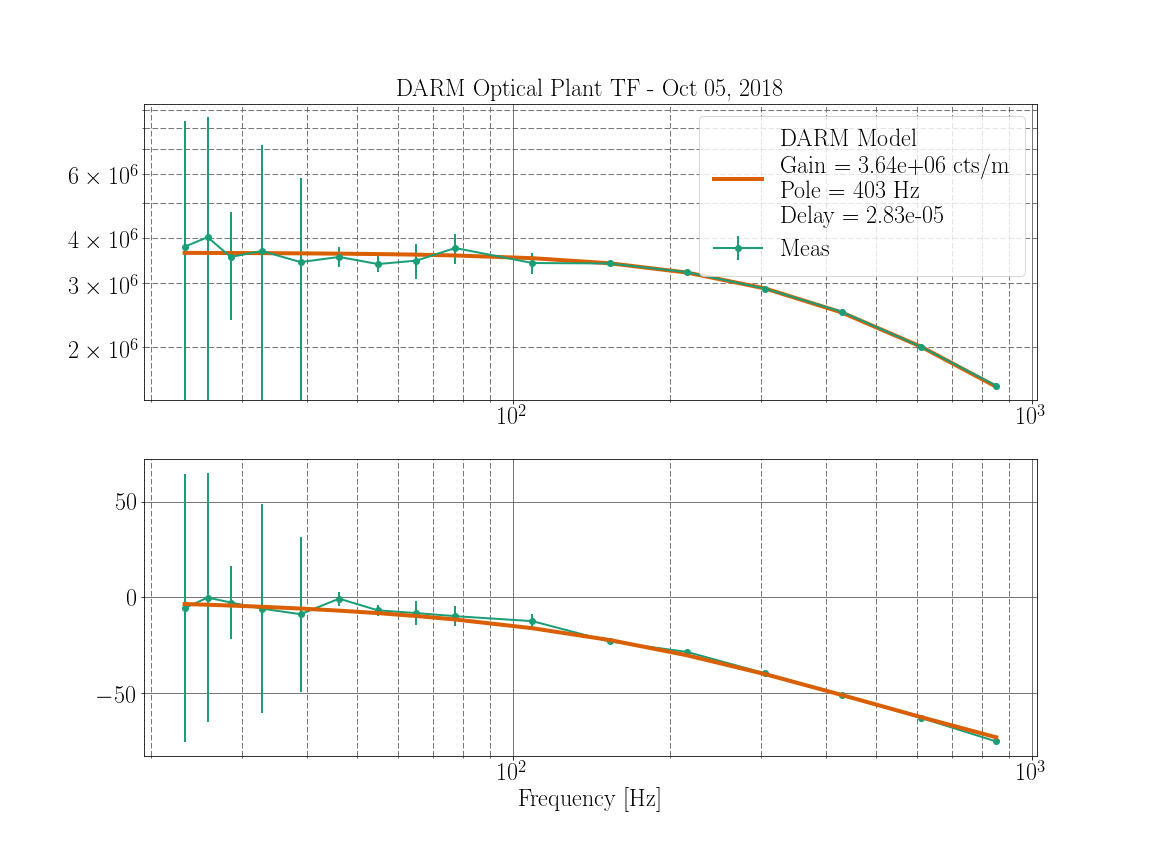
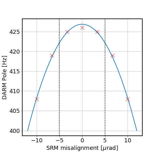
Our DARM shot noise calibration has been off by a factor of 4. I took a PCAL to DARM sweep and DARM OLG and got a rough measurement of the DARM optical plant while locked at 10 W. Templates saved in/ligo/svncommon/CalSVN/aligocalibration/trunk/Runs/O3/H1/Measurements/FullIFOSensingTFs/. I then fit a simple pole model to the measurement:Gain: 3.642e6 cts/m (cts are DARM error cts) Pole: 381.83 HzOur expected DARM pole with 32.3% SRM transmission is 433 Hz, so we are 12% low. Our SRC is poorly aligned, though, and the SRC ASC loops were off during this measurement. According to Hang's SRC misalignment simulation, if SRM misalignment was totally responsible for this low of a DARM pole, the SRM would be far more than 10 microradians misaligned, which is probably not the case. Another culprit could be ITM differential lensing, which is high for us right now. Together these could explain our measured DARM pole. I added new filters in the CAL-CS_DARM_ERR filter module to put our latest inverse sensing calibration into the front end:O3_D2N: zpk([382.0;6.7496;-7.0660],[0.1;0.1;7000],1,"n")gain(4768.4) O3Gain: gain(2.7473e-07)We have a dip at 180 Hz because we haven't updated the control signal calibration yet. Edit: Also interesting is jitter at 300-350 Hz appears to be reduced.
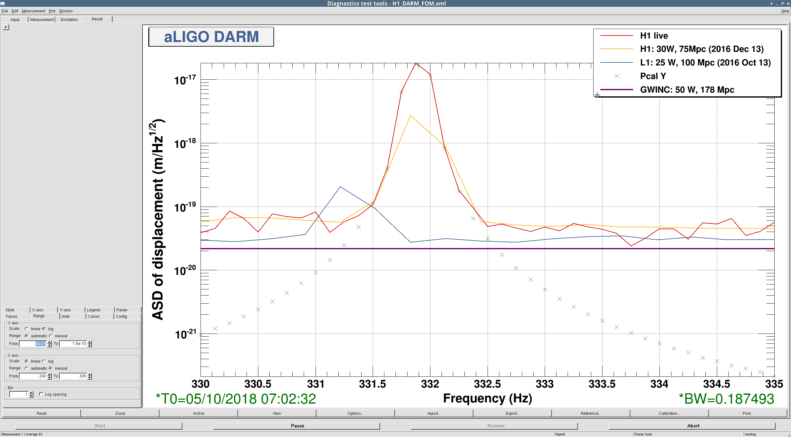
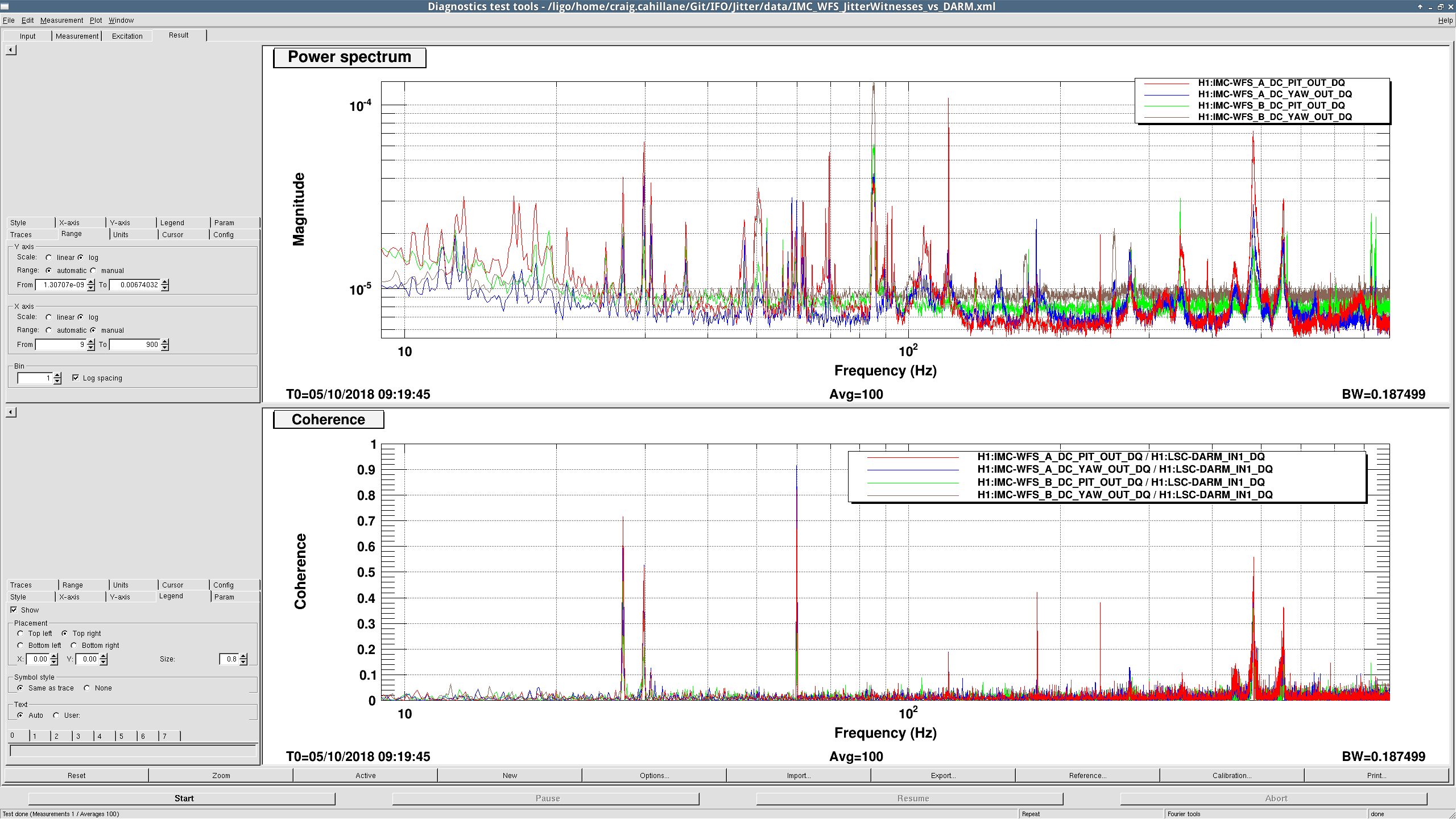
Robert, Craig We looked coherence between DARM and the IMC WFS jitter witnesses at the time of the 10 W spectrum from last night. The broad humps at 300-350 Hz are notably absent, and some jitter peaks (483.1 Hz and 553.5 Hz) are still present and reduced. We will reveal more when we go to higher power.
Improved single DARM pole fit and added delay parameter. DARM pole is actually 403 Hz, delay is 28 microseconds, gain is 3.64 cts/m. Calibration group will post full model fit shortly.
Craig, Sheila, Georgia
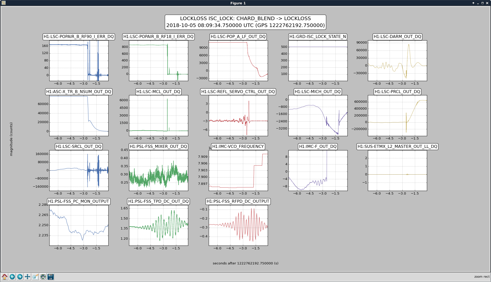
This evening we had a fast lockloss from 10W. The IMC did not lose lock however we saw on the beam on the reference cavity reflection and transmission cameras jiggling at something like 3Hz, as if the ref cav was swinging around.
We ran the lockloss tool and included some PSL channels; sure enough see a 3Hz oscillation in the ref cav transmission and reflection, starting 3 seconds before the lockloss. The oscillation is just visible in the IMC-F, but we don't see it in the mixer, vco, or eom monitors (see bottom two rows of plots in the attachment).
Maybe this is a clue for our past fast locklosses?
I looked into the source of the reference cavity motion and loss of lock and found that it was a huge site-wide but rare seismic and acoustic event. The interesting thing is that the arrival time at all stations is within about a second. This is consistent with teleseismic events, but unlike an earthquake, it has content up to 30 Hz (Figure), which should be highly attenuated for distant seismic signals. It is unlikely to be something nearby generated at the surface because the propagation delay is too small for surface waves of these frequencies. It would have to be generated right out in the middle of the arms at nearly the same distance from each of the buildings. It could be a small earthquake located nearly right under us.
It could also be acoustic, but it would have to originate far above us to be consistent with propagation delays. I think it is most likely under us because the seismic SNR is higher than the acoustic SNR. Also, the TF signature is not consistent with flying vehicles.
In any case, the DV plot in the figure shows that it is rare, nothing else as loud in the last month.
We tested again the digital compensation of the Sidles-Sigg torque at 10 W.
========================================================
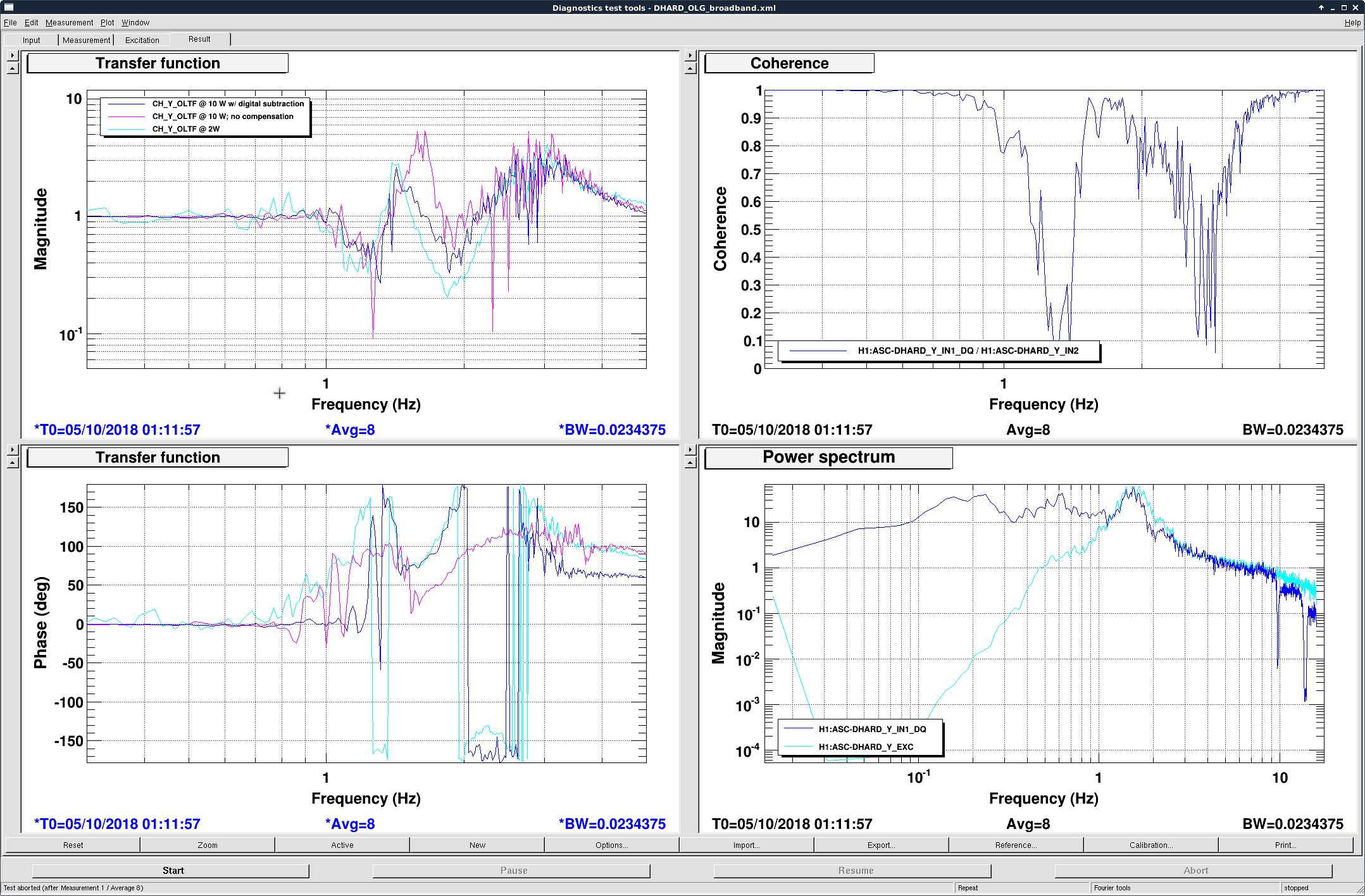
For yaw the subtraction was pretty successful. Please see the first attached image.
The cyan trace is the DHARD YAW OLTF measured at 2 W.
The pink is the OLTF measured at 10 W without any digital subtraction. We can see the OLTF changes as the radiation torque modifies the plant.
Lastly the blue is the OLTF for DHARD YAW still measured at 10 W, but this time with a digital path to create a torque canceling the radiation torque from the Sidles-Sigg effect. It successfully reduced the OLTF to look like the 2 W one. The gain for the subtraction at 10 W is -0.8, and we expect it to scale roughly linearly with respect to the arm circulating power.
========================================================
Although yaw was successful, pitch was not. As we tune the gain for the subtraction path we saw in the DHARD PIT error peak a peak showing up at ~ 0.8 Hz or so, consistent with the main resonance frequency shifted by the radiation pressure. The same peak did not show up if we did not turning on the compensation, indicating it should be suppressed by the ctrl loop. Thus we suspect the original of the peak was due to I poorly measured the sus plant and the fitted main resonance peak was slightly off compared to the real one. As we subtract two resonant peaks with slightly shifted frequencies, we created a sharp zero in the OLTF. The peak then caused strong gain peaking in the closed loop system.
The solution is therefore to take a more careful measurement of both the L2 torque to L3 pitch, and the L3 torque to L3 pitch suspension plants.
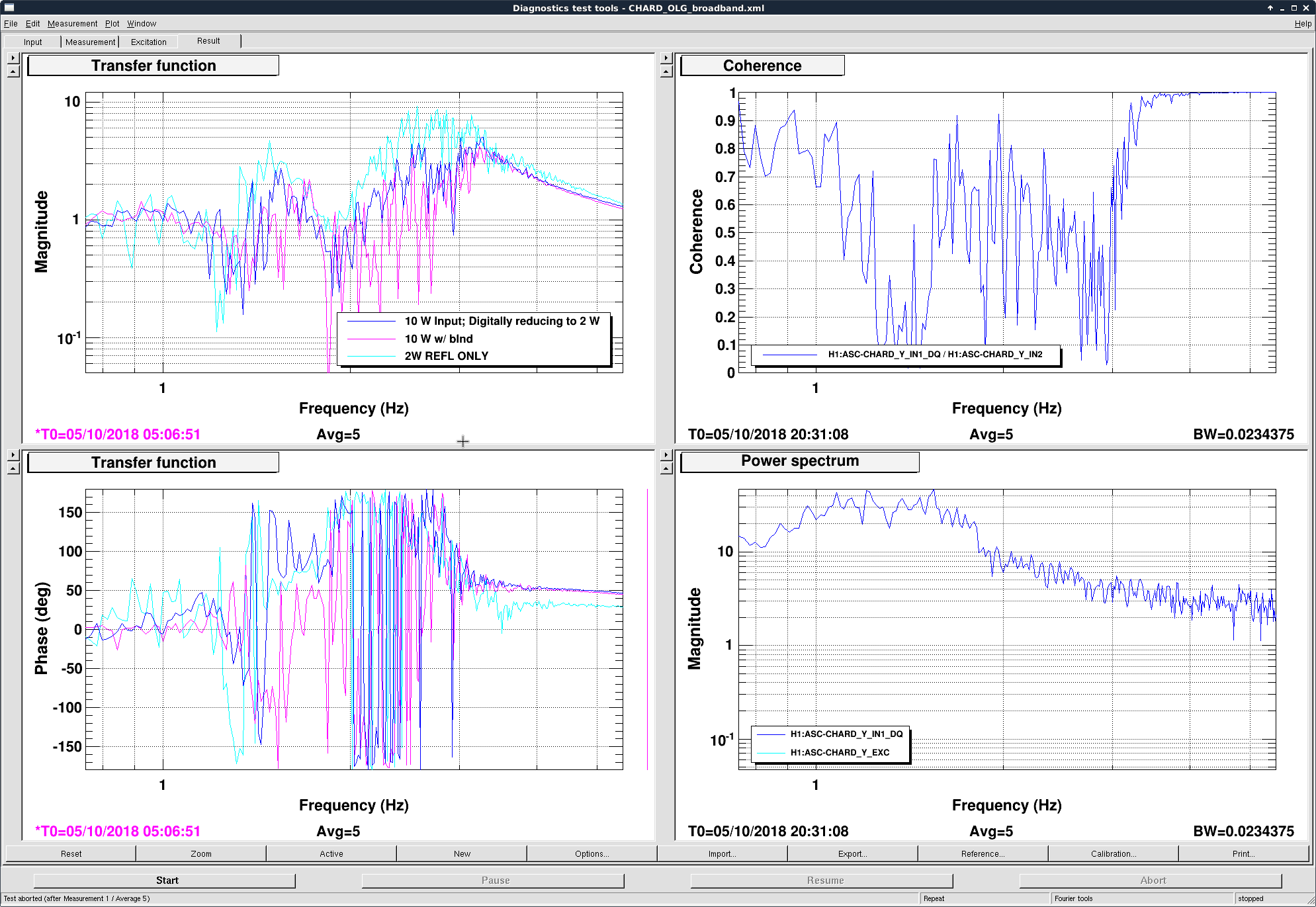
Attached is the similar plot for CHARD YAW. Due to the fast lock losses we could not get more averages to clean up the plot, yet it seemed that the compensation is making the CHARD YAW OLTF closer to the 2W one. Maybe we are a bit under compensating, but as we are creating a digital soft mode (which by itself destabilizes the loop) to cancel the hard mode, it is safer to under subtracting then over subtracting.
The error signal we used is the same blended CHARD YAW error signal as currently used in the regular ASC ctrl loop. As above 0.4 Hz the error signal is essentially from the TR QPDs, which are clean signals sensitive only to the ARM DOFs but not the corner ones, we should expect it work as good as DHARD. The ASC-RPC_CHARD_Y_GAIN used for this plot is +0.8 and should scale roughly linearly with input power. I.e., roughly the gain should be +0.8 * (input power / 10 W), though we still need some fine-tuning as the optical response (which we need to calibrate the cts input back to physical CHARD radians) may change wrt the input power.