peter.king@LIGO.ORG - posted 05:21, Tuesday 20 December 2016 (32765)
OSB parking lot
The OSB parking lot is slippery as a skating rink out there. Exercise caution.
The OSB parking lot is slippery as a skating rink out there. Exercise caution.
10:44:24UTC
Even more reason to have that sleeping trailer back!!
TITLE: 12/20 Eve Shift: 00:00-08:00 UTC (16:00-00:00 PST), all times posted in UTC
STATE of H1: Corrective Maintenance
INCOMING OPERATOR: Ed
SHIFT SUMMARY: After two attempts of initial alignments, the alignment looks okay now. First lock attempt I went all the way to PRMI LOCKED without a problem (until I moved a wrong optic and broke lock, that optic was moved back). Now it won't even get passed Locking ALS. It kept breaking lock at ALS DIFF. I followed Jenne's document and checked ETMX ESD settings. Everything looks fine.
After Jeff and I struggled to get a good Y-arm alignment earlier this evening due to weird fringes, I managed to get rid of them by moving BS in yaw (this is after I put it back to where it was -20 hours ago which I thought was a good alignment). This make senses if the ALS camera locate in the corner station (is it?). It's a small victory of the night. Now moving on.
Meanwhile more earthquakes from Greece and Papua New Guinea have arrived.
5.1M Vanuatu
Was it reported by Terramon, USGS, SEISMON? Yes, Yes, No
Magnitude (according to Terramon, USGS, SEISMO): 5.1, 5.1, NA
Location (according to Terramon, USGS, SEISMON): Port-Olry, Vanuatu
Starting time of event (ie. when BLRMS started to increase on DMT on the wall): ~4:30 UTC
Lock status? Unlocked
EQ reported by Terramon BEFORE it actually arrived? Terramon page loaded AFTER the earthquake has arrived.
6.4M Solomon Islands
Was it reported by Terramon, USGS, SEISMON? Yes, Yes, No
Magnitude (according to Terramon, USGS, SEISMO): 6.4, 6.4, NA
Location (according to Terramon, USGS, SEISMON): Kirakira, Solomon Islands
Starting time of event (ie. when BLRMS started to increase on DMT on the wall): 4:48 UTC
Lock status? Unlocked
EQ reported by Terramon BEFORE it actually arrived? Terramon page loaded AFTER the earthquake has arrived.
6.7M Solomon Islands (Terramon only)
Was it reported by Terramon, USGS, SEISMON? Yes, No, No
Magnitude (according to Terramon, USGS, SEISMO): 6.4, NA, NA
Location (according to Terramon, USGS, SEISMON): Kirakira, Solomon Islands
Starting time of event (ie. when BLRMS started to increase on DMT on the wall): 5:09 UTC
Lock status? Unlocked
EQ reported by Terramon BEFORE it actually arrived? Terramon page loaded AFTER the earthquake has arrived.
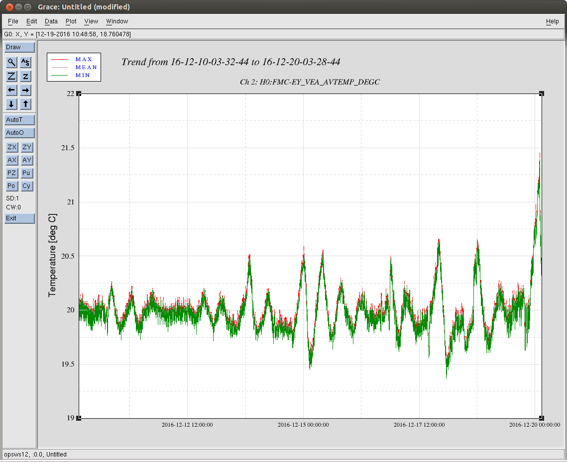
J. Kissel, N. Kijbunchoo

We're on level three distraction from what we believe is our potentially main issue/problem:
- (Level 1) We started hoping to return to nominal low noise ASAP to test whether the ETMY PUM/L2 stage coil driver swap has improved the recent plague of glitches, and/or changed that stage's coil balancing, length-to-pitch plant, or actuation strength.
- (Level 2) We then had trouble with ALS losing lock constantly before finding IR. So, we spent a few hours just going through ALS locking steps one at a time in hopes to find a specific problem. This go us no where, and as per typical, we got lucky once and made it past all the way up through COIL_DRIVERS after DC_READOUT and POWER UP. We saw an oscillation in IFO signals eventually lead to a lock loss.
- After failing again at ALS, we decided it must be initial alignment (given evidence of low green power from the X Arm).
- (Level 3) Once finished with the first round of initial alignment (which took particularly long because SR2 was in the wrong spot), we found the Y-arm totally hosed in alignment.

Now, Nutsinee and I are just chasing our tails with the Y arm green locking, likely because of the 2 [deg] C temperature swing of the YVEA after the chiller failure.

I'm going home, Nutsinee's just going to wait it out until the temperature returns to normal.
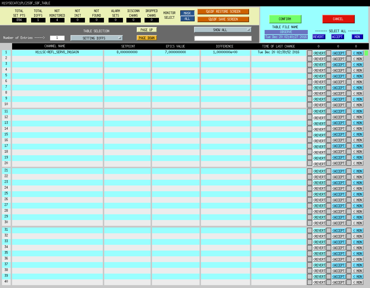
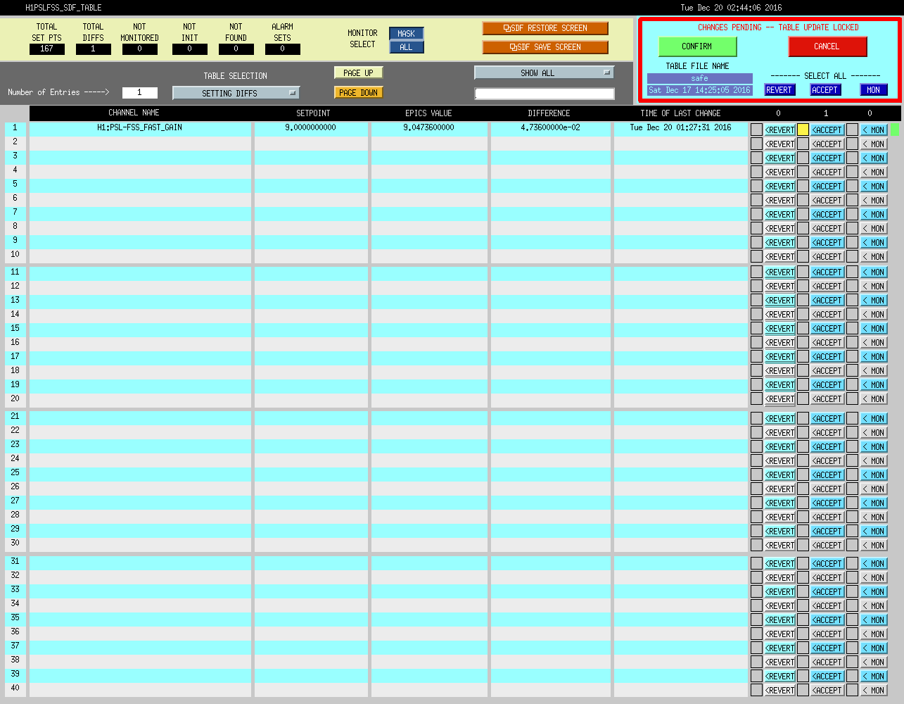
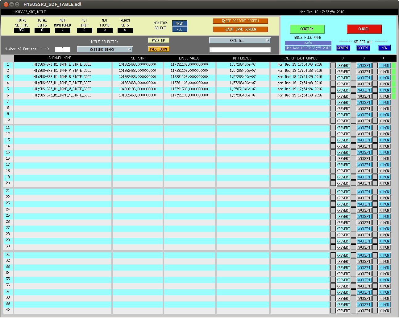
J. Kissel

While Nutsinee and I were trying to debug why SRCL would not trigger during SRY initial alignment sequence, I noticed that SR3's ODC vector showed red. As I've seen in several suspensions, it was the comparison between a user-entered-but-rarely-paid-attention-to "H1:SUS-SR3_M1_DAMP_[DOF]_STATE_GOOD" channel that was not set to match the current state of the filters, "H1:SUS-SR3_M1_DAMP_[NOW]_STATE_NOW."
This appears to have gone bad on Nov 17 2016 00:26 UTC (Nov 16 2016 16:26:00 PST), when Sheila added highest vertical and roll mode notches for the HLTS -- see LHO aLOG 31553.

Fixed now. Doesn't matter, but one less bit of red to distract people.

Changes have been accepted in the SDF system in both the SAFE and OBSERVE.snaps.

It looks like the EY chiller 2 has tripped. I have started the alternate water pump (CWP1) in order to enable chiller 1.


J. Kissel, N. Kijbunchoo

Found ALS Fiber Polarization high at ~20% for X Arm Fiber PLL. Went to CER and reduced it. Couldn't get better than ~9%, but should be good enough.
(see Dave B's entry @ https://alog.ligo-wa.caltech.edu/aLOG/index.php?callRep=32741)
TITLE: 12/19 Day Shift: 16:00-00:00 UTC (08:00-16:00 PST), all times posted in UTC
STATE of H1: Observing at 66.0999Mpc
INCOMING OPERATOR: Nutsinee
SHIFT SUMMARY:
A bit of a slog. H1 was locked for a few hours at the beginning of the shift and then taken down (while L1 was down) to swap the ETMy L2 Coil Driver. This was thought to be the suspect of our glitchy H1. But we might be finding out that swapping this out might not be trivial.
LOG:
J. Kissel, J. Driggers, C. Gray

Ever since the sudden drop in X-arm green laser power in Oct 2016 LHO aLOG 30884, it's been a challenge to pass the metric for determining whether the arms are locked well enough to begin locking ALS -- if ALS-C_TRX_A_LF_OUTMON and ALS-C_TRY_A_LF_OUTMON are greater than 0.9 (normalized [ct]). However, we often see via other metrics that the arms have settled and are in a fine enough condition to move through ALS.

As such, we've lowered the threshold on X arm transmission to 0.85.

This is modification to the
/opt/rtcds/userapps/release/isc/h1/guardian/ISC_library.py
The change has been committed to the repository.
What is going on to explain the exhaust pressures depicted in the attached?
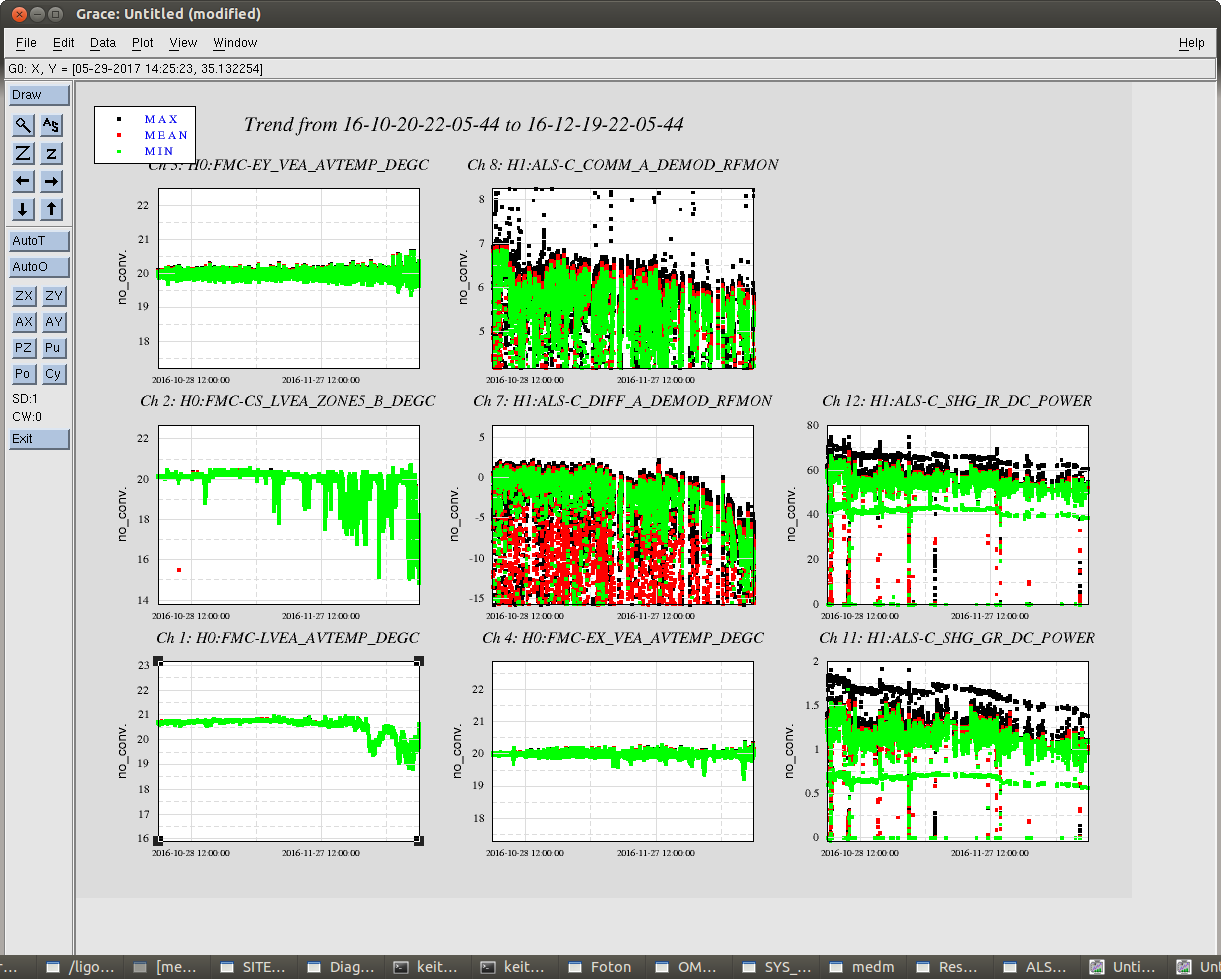
It seems like the LVEA temperature is not as stable as it should be, and among other things this might be correlated to the slow trend of ALS diff signal going down. It used to be 0dBm, now it's -8 to -10 dBm.
Since diff (X-Y) is degrading much faster than comm (X-SHG), and since it's degrading faster than the SHG power, this is probably just an alignment of some steering mirror on ISCT1. This needs to be fixed tomorrow during the maintenance.
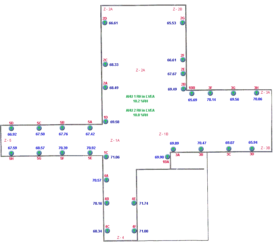
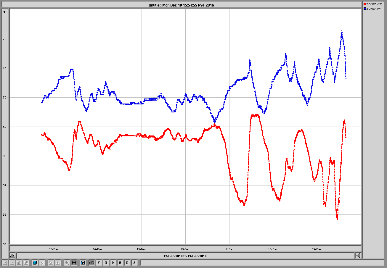
Keita and I looked at zones 4 and 5 temperatures (Output MC and Input MC ) and noticed that they are oscillating in opposition.
In response I have done the following;
Reduced heat zone 3A (from 10ma to 4ma) - this is a reduction of ~33kw or one stage of a 3 stage heater.
Reduced heat zone 5 (from 10ma to 8ma) - Variac controlled - not sure of the power reduction but duct temperature dropped by ~5 degF.
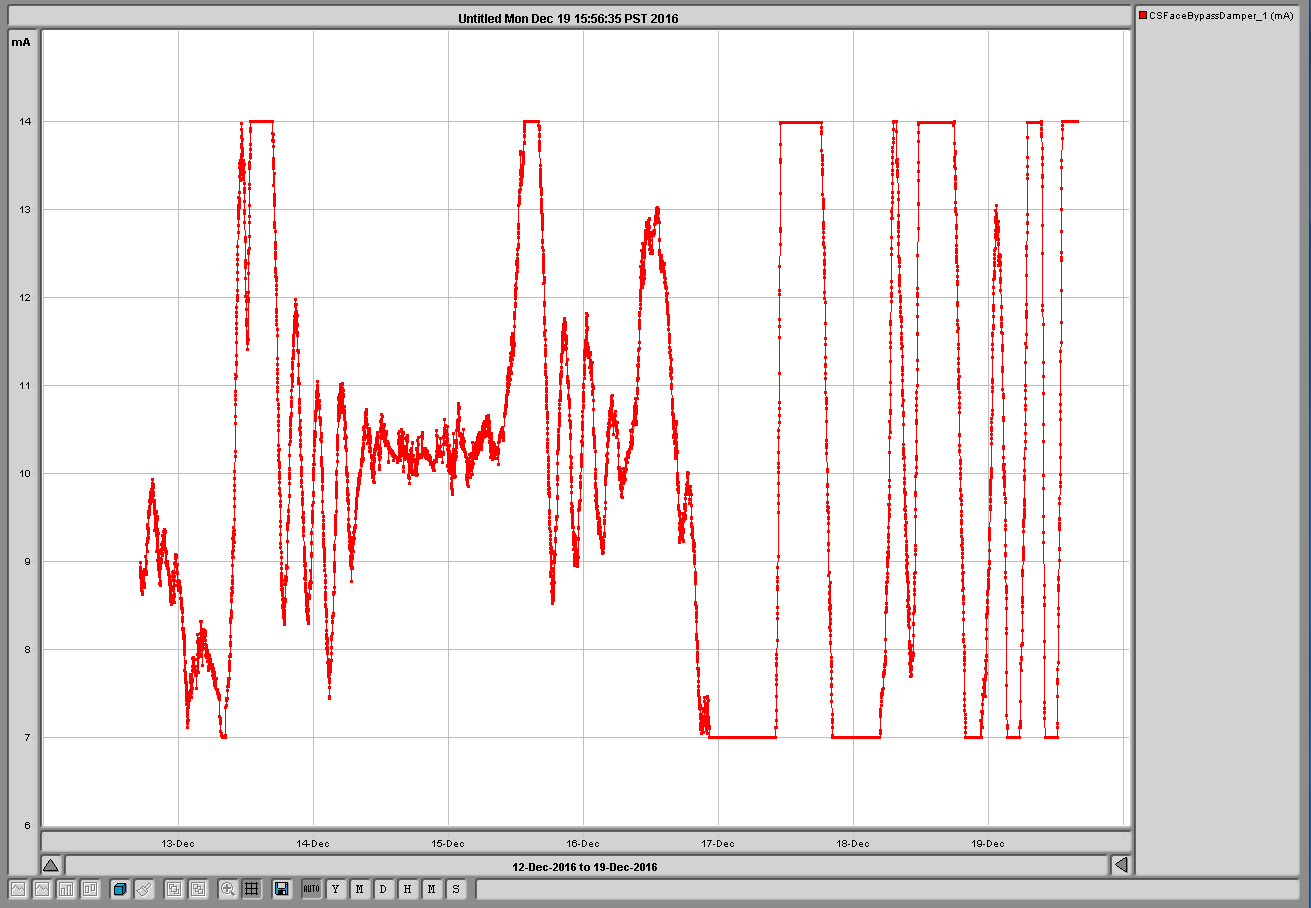
Reduced chilled water setpoint to 43F from 47F to provide more control authority for the chilled air portion of the air handler. The face bypass damper has been swinging from rail to rail for the last few days.
No warranties are implied.
Bubba and I will continue to monitor and adjust.
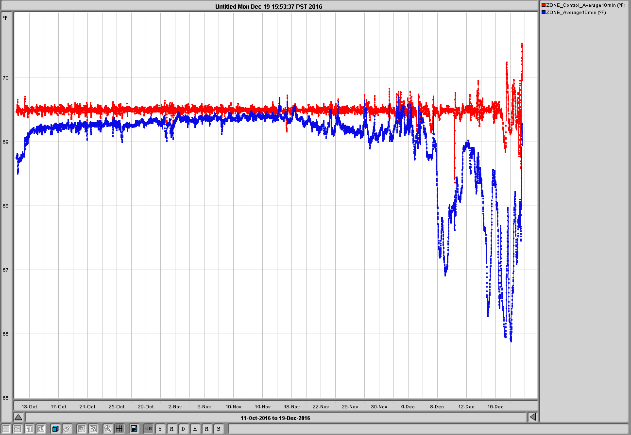
Temperature of the LVEA is controlled based on the average called H0:FMC-LVEA_CONTROL_AVTEMP. Don't expect H0:FMC-LVEA_AVTEMP to behave as nicely.
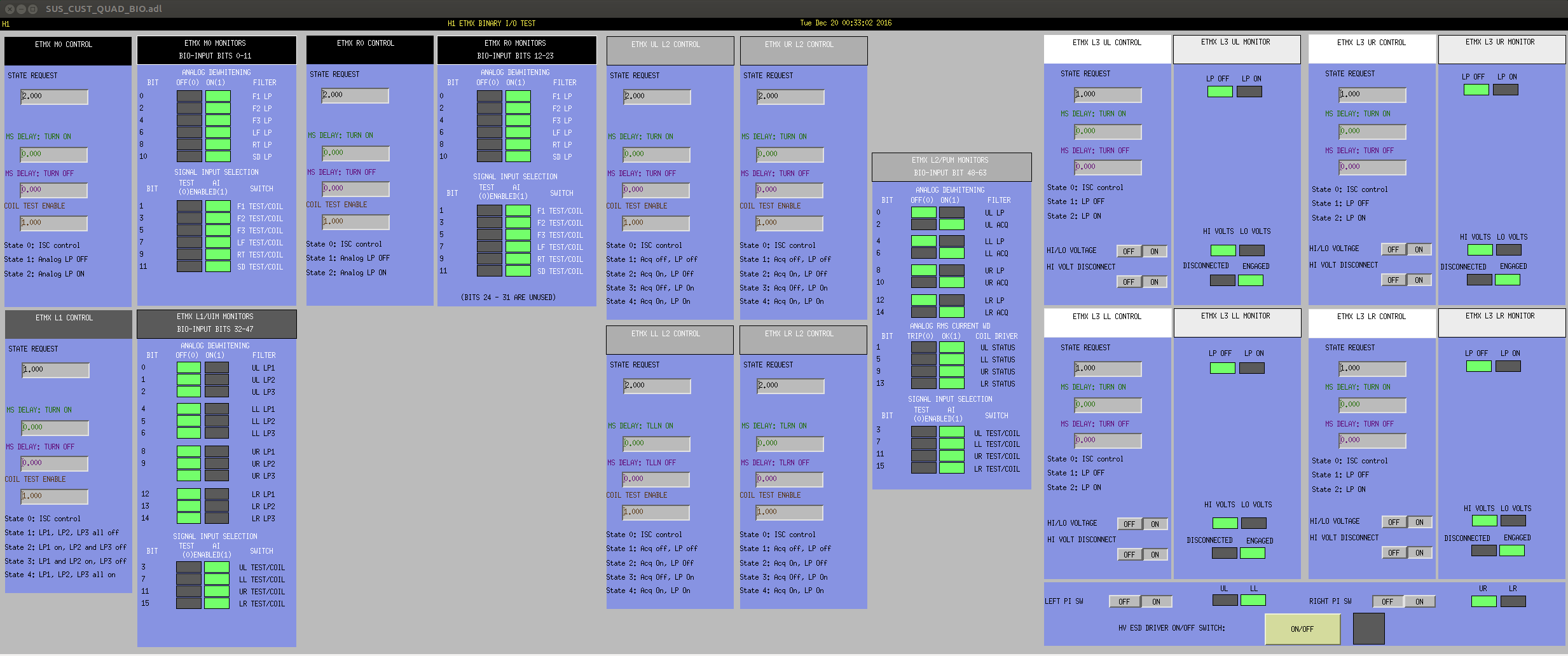
Alog entry from DetChar points to ETM PUM chassis as a possible source for the glitchiness seen over the lock stretches. Robert Schofield says magnetometer in ETM SUS rack confirms glitchiness is coming from inside rack. This morning we replaced PUM S1102652 with S1102648.
Tagging CAL. Also DetChar so they're aware the change was made and what collateral damage occurs after potentially fixing zee glitching.

This change can potentially affect the calibration of the IFO at low frequency, since we use ETMY during nominal low-noise control. In order to quantify this, we're going to take an L2/PUM stage actuation strength sweep once we get the IFO back up and running. Then, tomorrow during maintenance, we'll re-measure the chassis alone to check if all poles and zeros of the filtering need to be re-compensated as we'd done back in May 2016 (see LHO aLOG 27180 and 21232).

If there is a significant change in the frequency dependence then we must update the PUM stage compensation filters (and no change will be necessary to the calibration). If there is a significant change to the actuation strength, then we'll need to change the actuation strength of L2 stage in the front-end CAL-CS model.

Further, the coil balancing for each stage will potentially be different as well. So we may need to resurrect re-balance the coils a. la. LHO aLOG 11392. I sincerely hope we don't have to change any of the finely tuned L2P or L2Y filters that are in place in the L2_DRIVEALIGN_L2P and L2_DRIVEALIGN_L2Y banks. I can't find the original design aLOG, but Sheila found that the L2 L2Y filter doesn't do anything back in March of 2015 LHO aLOG 17322, so I suspect only L2 L2P may need to be adjusted. Hopefully some remembers how that filter was designed.
