Dave, Kiwamu, Nutsinee
--------------------------------------------------------------------------------------------------------
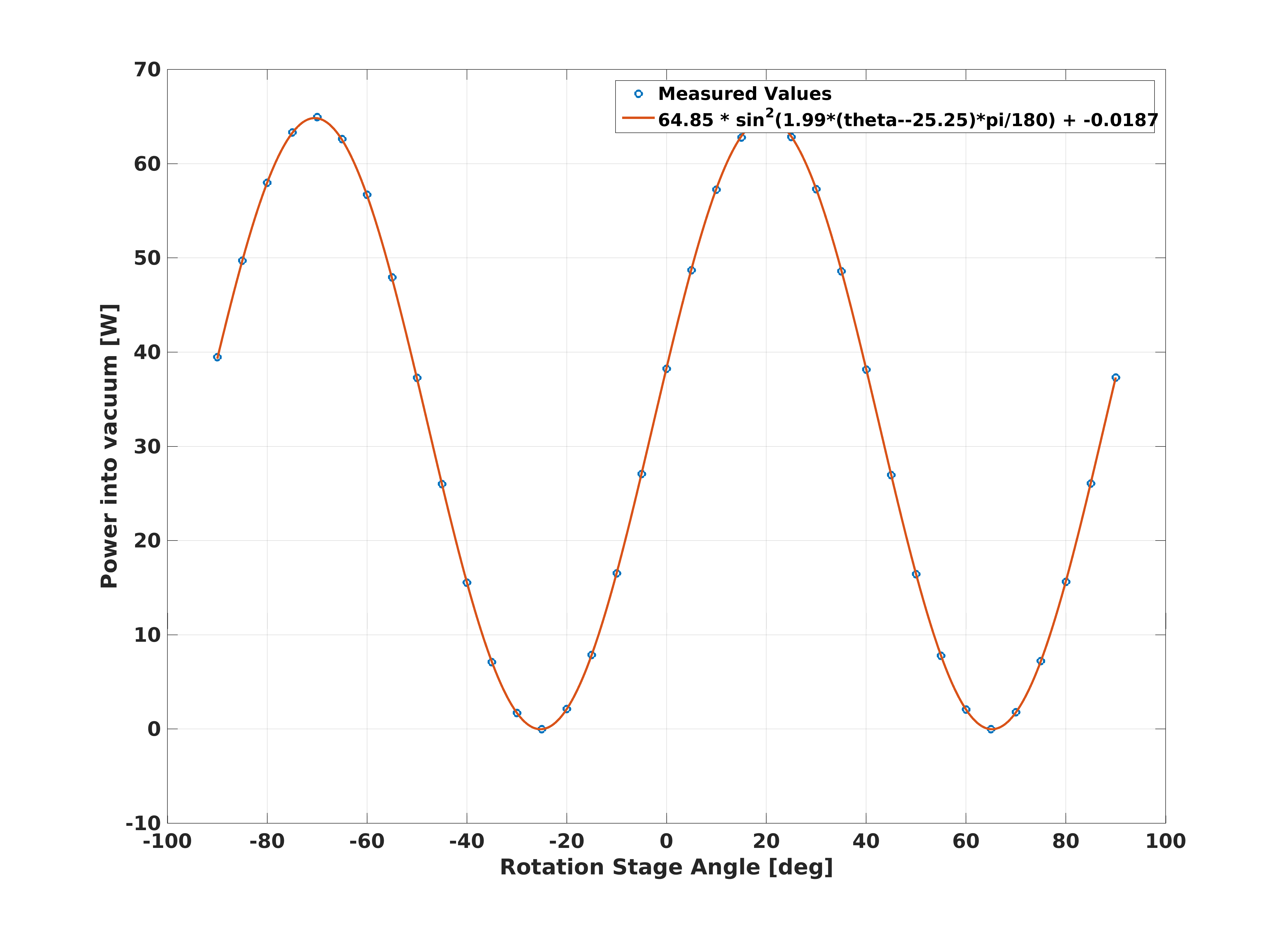
Quick conclusion: It's probably related to the CO2Y rotation stage.
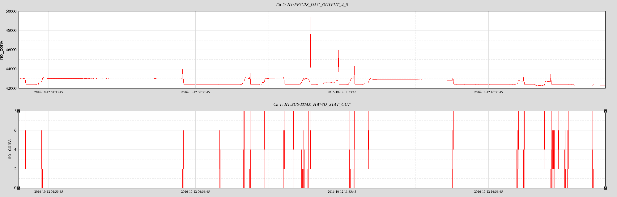
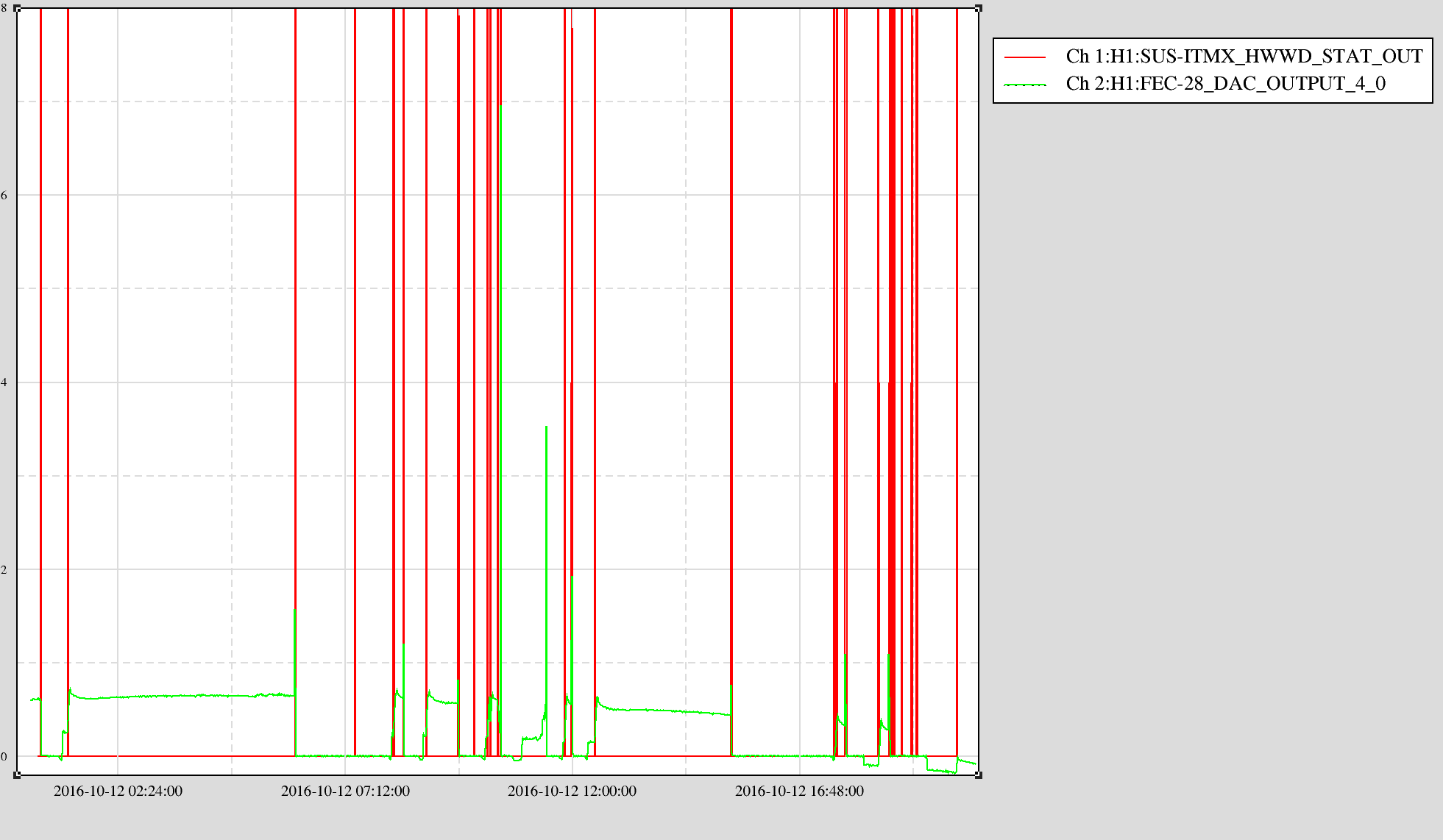
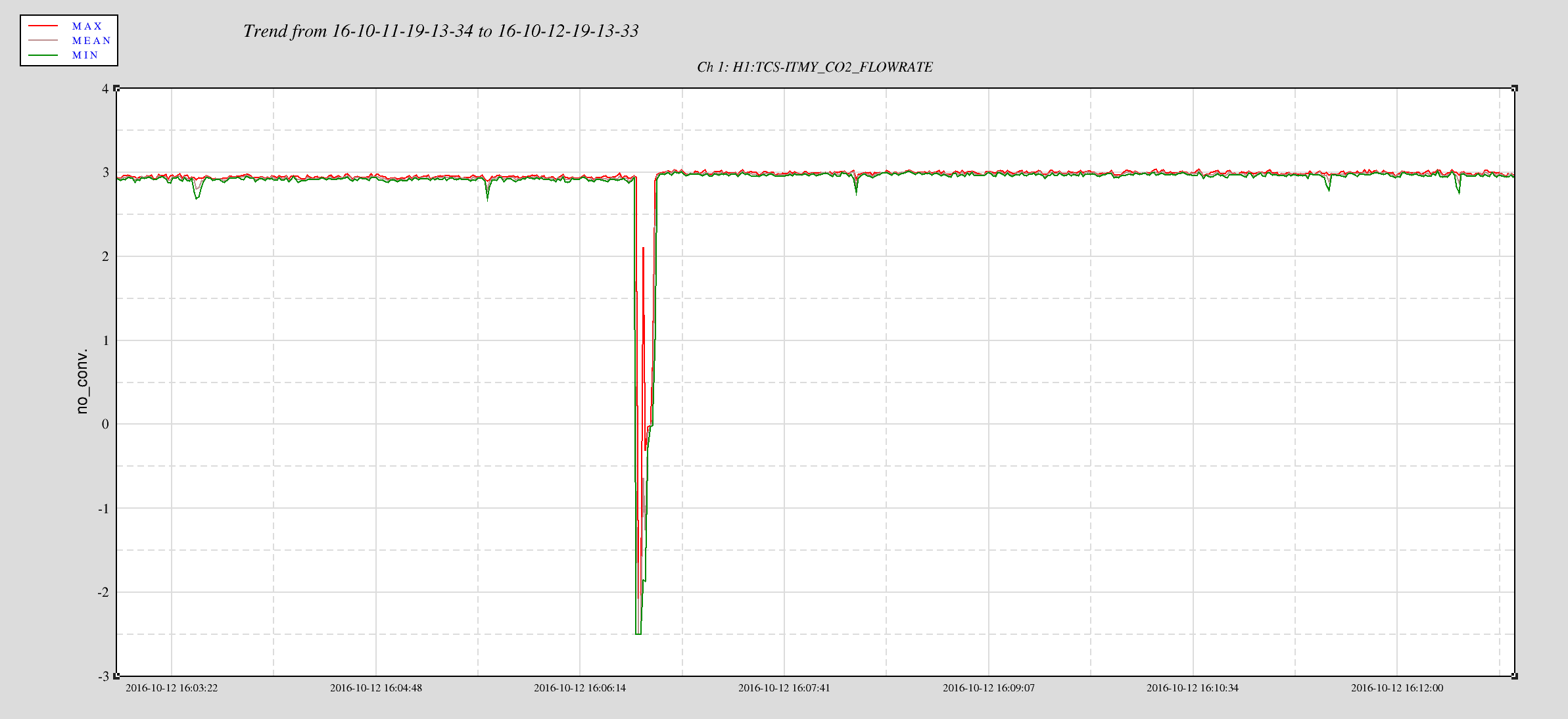
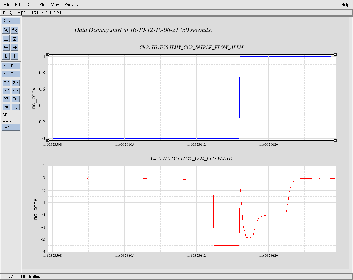
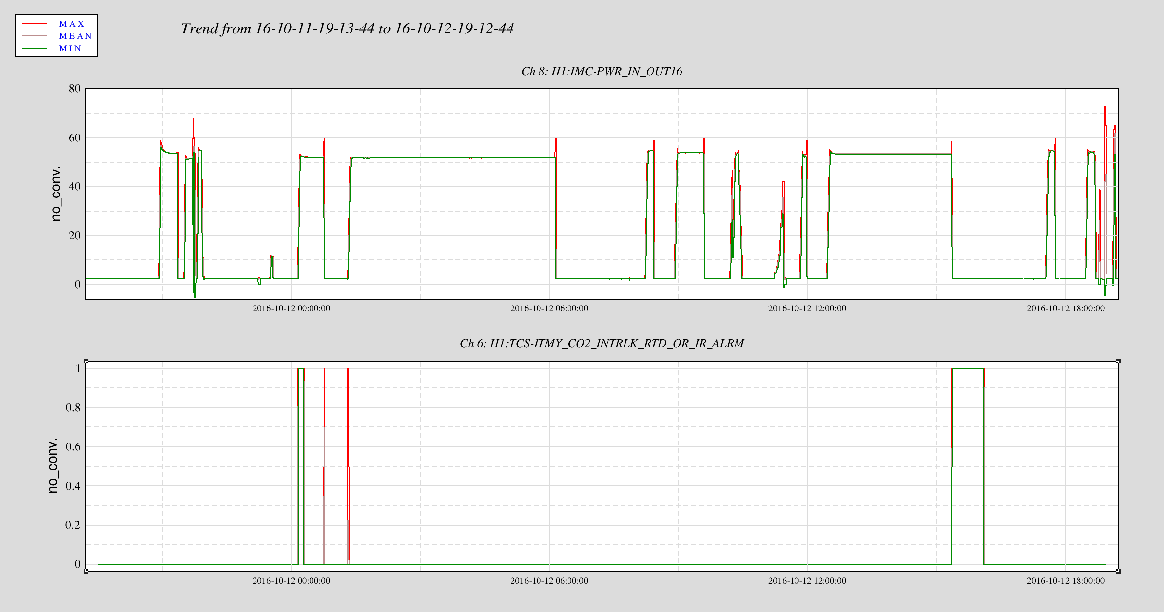
Lengthy details: Dave notcied TCSY chiller DAC output went crazy yesterday. After making sure that it wasn't the model update (alog30429, alog30384) that did it we investigated further. The crazy output to the chiller was due to TCS guardian trying to lock the laser when there were no laser (as the result the guadian keeps increasing and decrasing chiller temperature by about 1 deg C).
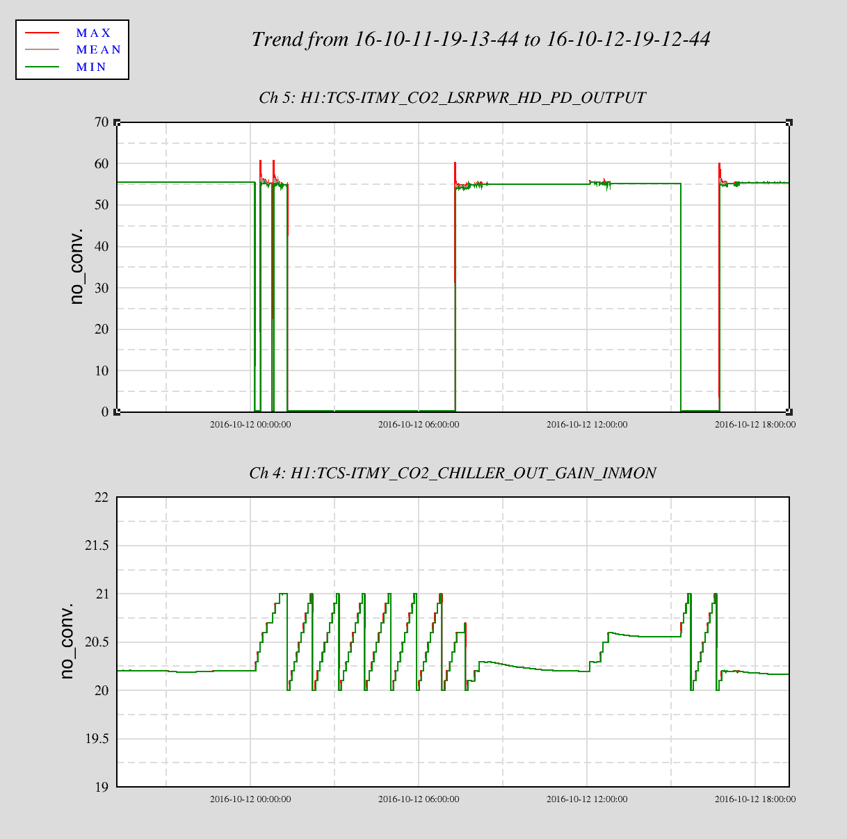
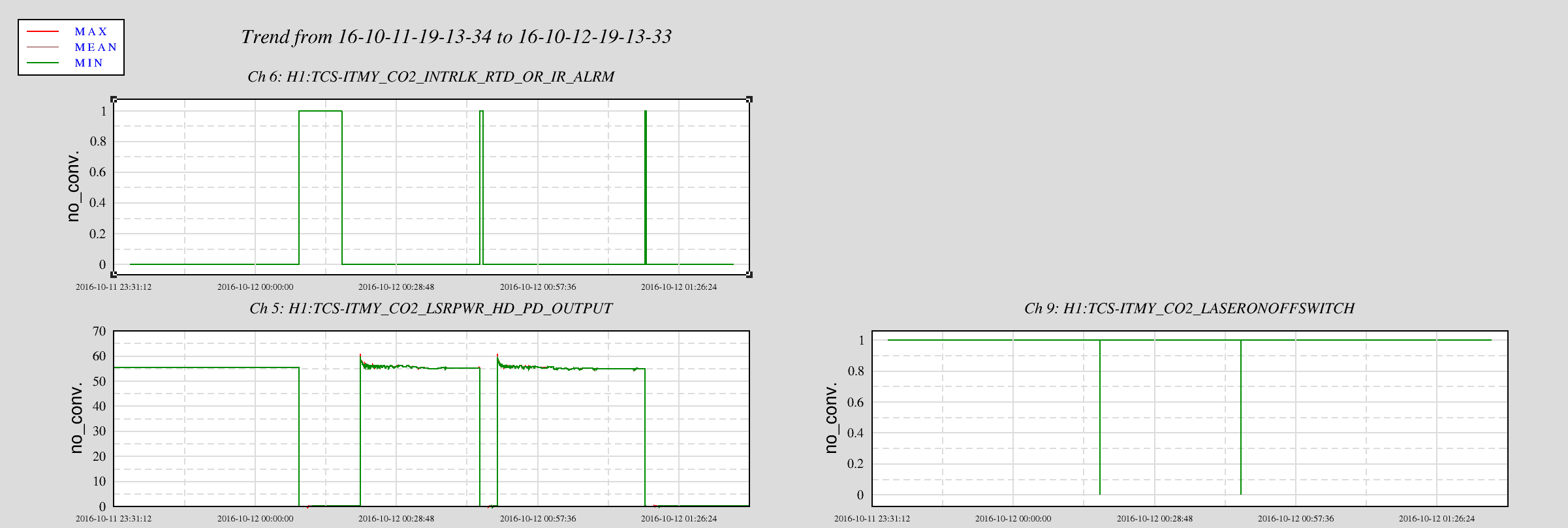
The cause of CO2 laser trips was due to RTD/IR ALARM interlock tripped, which always coincide with either power-up state and lockloss state. Although not every power-up or locklosses caused CO2Y to trip. We also looked at POP but it's not showing here.
This immediately made us think of the CO2Y rotation stage that would only move during these times. Could this be either Beckhoff or electronics issue? The fact that it actually tripped the interlock box made me think of grounding issue. But I always blame grounding.
Also Kiwamu was able to untrip the RTD/IR interlock and get the CO2 into "ready" state just by toggling LASER ON/OFF button. This is what we don't understand. How is this even possible?
The End.