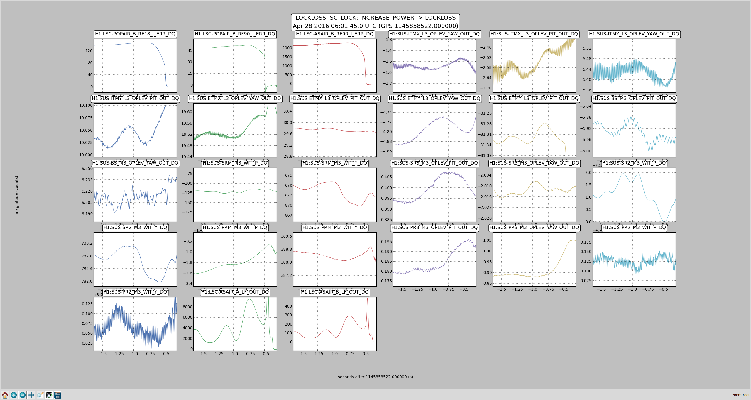
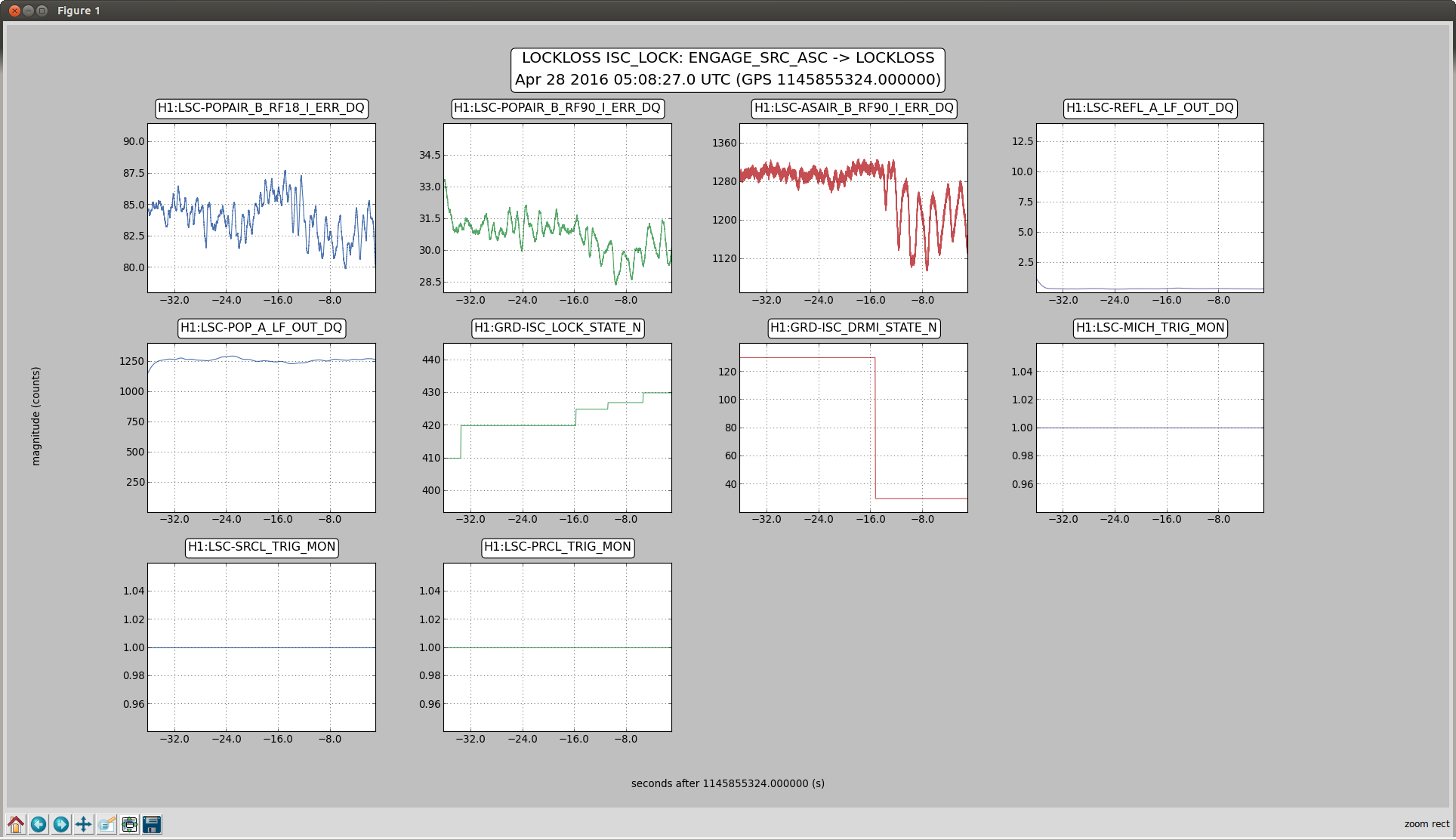
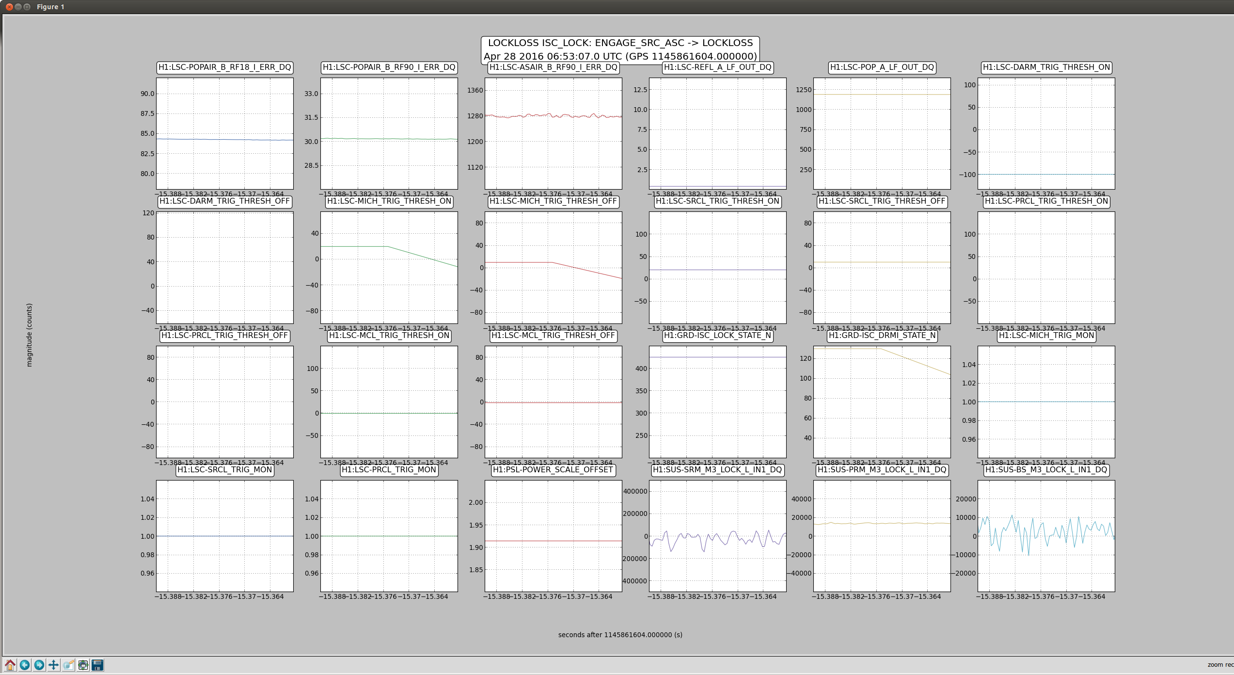
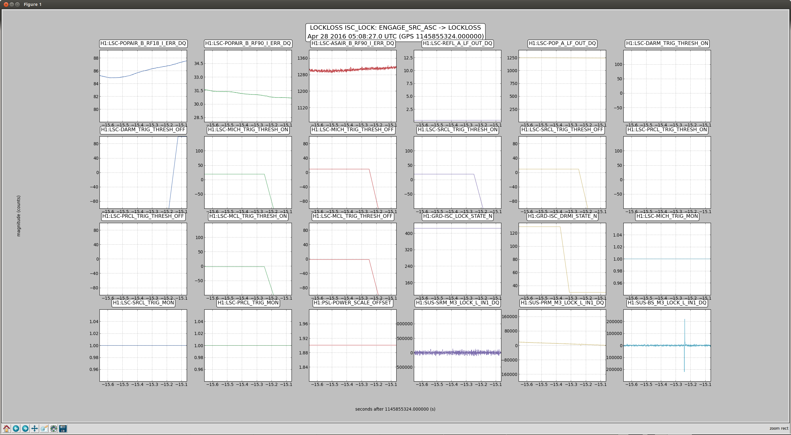
One of the lockloss classes from tonight has been some kind of angular instability that we see very strongly on the AS camera right when we start to power up. Not sure what it is, but it's the kind of thing that could be a BS angular instability, since the Michelson fringe separates, and the 2 bright spots orbit around each other for a second or so before we lose lock. It looks primarily like pitch according to the oplevs, but there are certainly some yaw components in there.
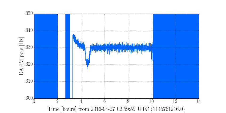
Attached is a plot showing the lockloss, including the power at the AS port and the oplev (or wit) signals from each of the IFO optics. If we call the frequency of the AS DC power fluctuations 2f, then it looks like perhaps BS and the ITMs are moving in pitch at 1f.
We tried once turning off the CHARD, MICH and SRC1 loops just before powering up. We were able to make it to 3W and sit for a few moments, but then lost lock on the way to 5W, although this was a fast lockloss, probably just because we didn't have enough loops on. We'd like to try powering up with all the loops on to 3W, to confirm that we can't even do that (we had always been going straight for 5W when we saw the instability). We'd also like to try with only 1 loop off at a time - MICH seems the most suspicious loop, but CHARD does seem to get noisy when the rotation stage is moving.
As a side note, I've added tried to add a convergence checker to the Engage_SRC_ASC state, so that you no longer have to wait by hand before going to Part1. You should be able to safely select Part1, and the guardian log will tell you what loop(s) aren't converged yet. The wait seems to not be working consistently yet, so maybe we can't depend on it yet, unfortunately.


The HWS is working nicely now. We see the ITMX thermal lens forming again.
Did the same for HWS-Y. Also reset the magnification to 7.5 instead of the default 17.5x