Times PST
7:40 Jeff B to LVEA for N2 dewar and CC work
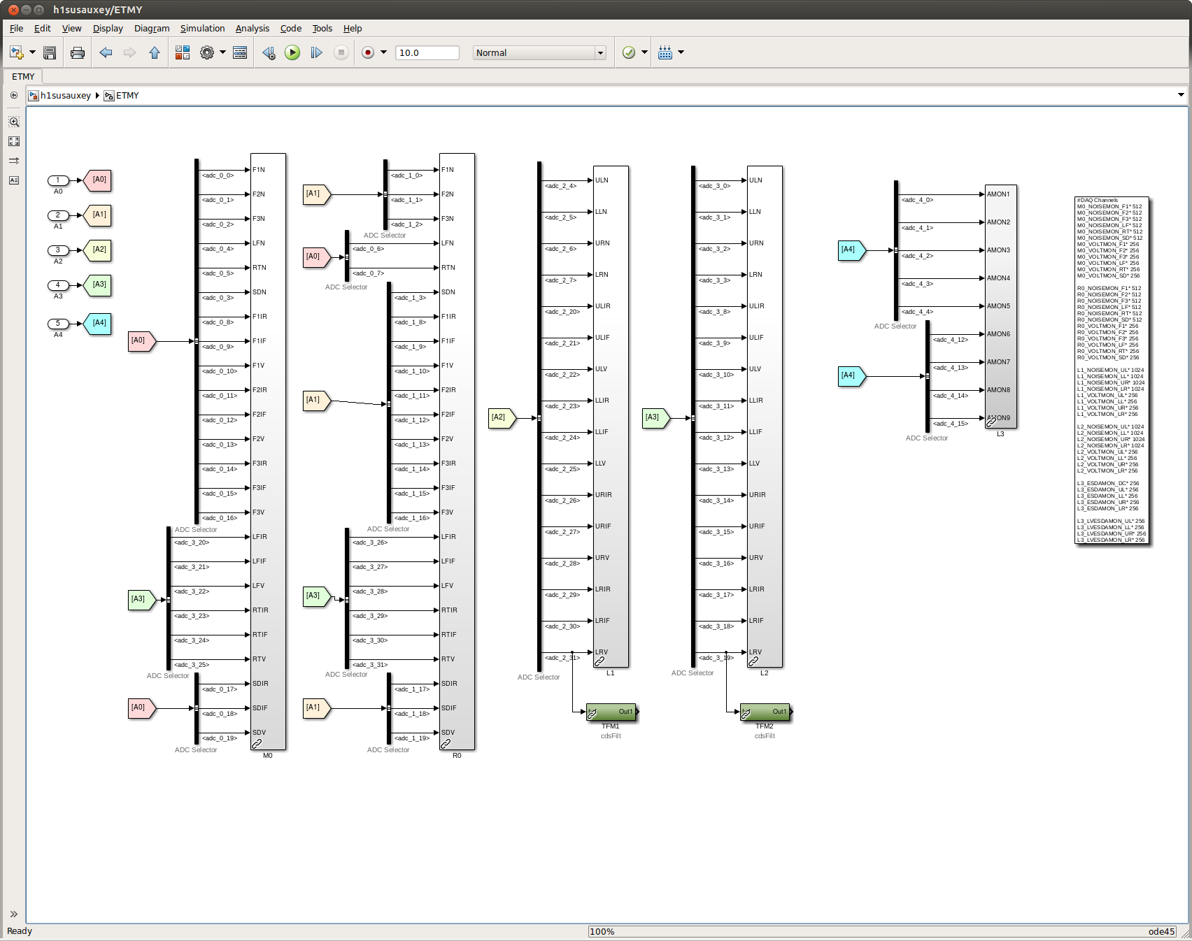
8:11 Jim B to EY for timing fanout and BIOS work
8:13 Jeff B done
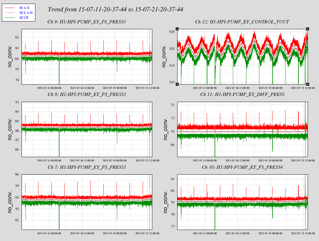
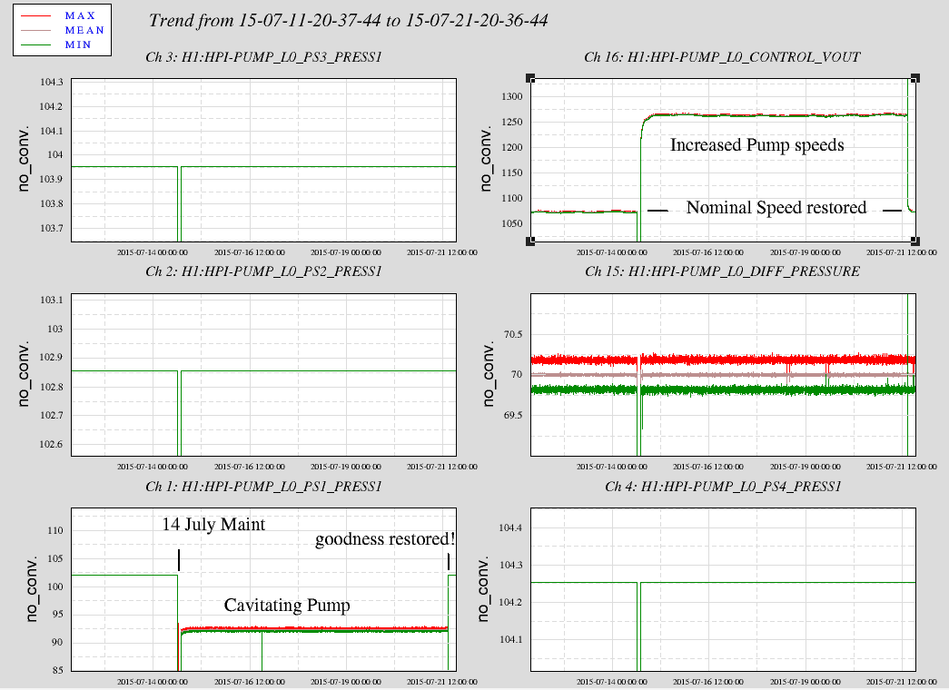
8:16 Hugh and Jim to HEPI mezzanine for pump station work
8:19 Andre to LVEA for cosmic ray detector cabling
8:20 Praxair on site
8:31 Vinny to EY for PEM work
8:33 Karen and Cristina to both ends
8:36 Kyle to both mid stations
9:00 Richard done w/ GPS work
9:15 Vinny to LVEA for tiltmeter work
9:23 Kyle back from mids, going to LVEA
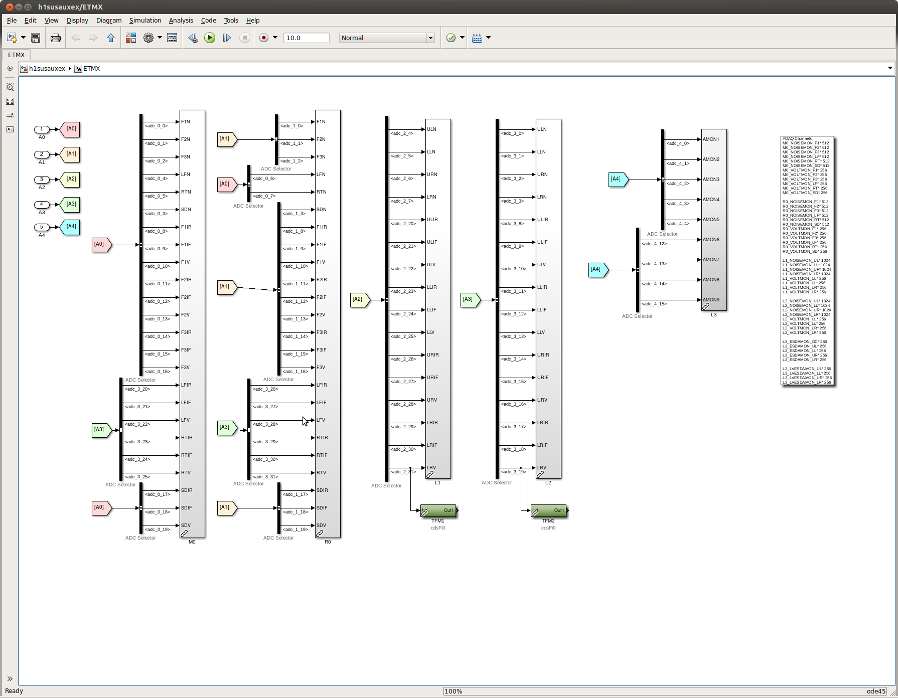
9:37 Jim B done at EY, going to EX for BIOS work
9:40 Dave doing EY software updates
9:48 Kyle done in LVEA
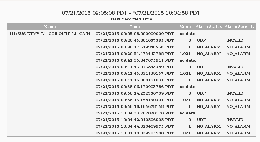
9:58 restarting EY SUS
10:00 Karen and Cristina done
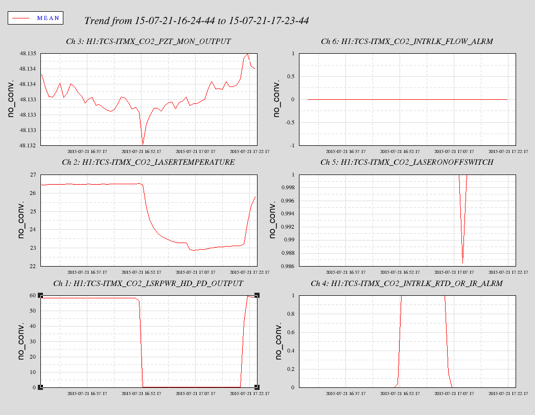
10:15 Nutsinee out to CER to reset TCS-X laser
10:20 Fil to EX for ESD LVLN install
10:38 Jim B done
10:45 Praxair on site
10:45 Kyle touring LN2 dewars
10:47 Hugh done
11:04 Nutsinee and Elli to LVEA TCS sensor check
11:38 Kyle done
12:08 DAQ restart
14:45 Dave to MX for PEM power supply replacement
14:52 Richard to CER
15:14 Dave back