Due to a mistake in past CHETA models there is more astigmatism then expected on the tables and a change in beam size at the ITM. The astigmatism can be fixed by rotating L1 around the vertical axis and the beam size can be changed by movind L2 using the translation stage in each setup. Using a modified Fintrace model the required rotation angle and translation for each table  as they are currently populated at LHO (0922, 0918) and LLO (0919, 0851) have been calculated and are shown below. 
The tables below give the current astigmatism and then the angles and translations such that the x and y beamsize on the ITM is 52.7mm with no astigmatism. 

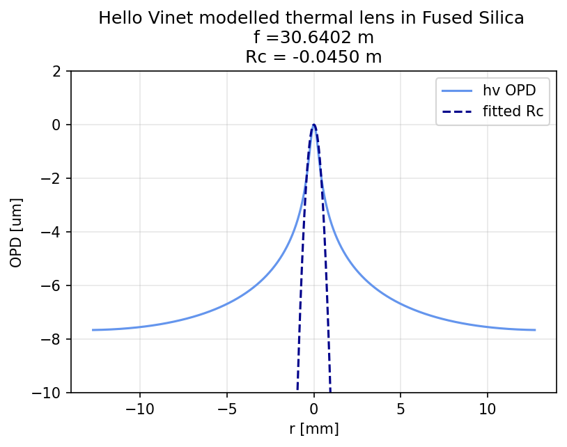
This code is avaliable in the CHETA modelling repository.

Without translating of L2 astigmatism can be removed but the beam size is still unoptimised.  

Sheila, Keita, Jennie W, Jenne D, Georgia B.

We want to be able to power up to 20W in JAC to check the POP beam.  

We were loosing lock with about 8W into JAC because the REFL shutter was closing.  Jennie Wright measured 6mW on the REFL diode with 2W input to HAM1 and JAC unlocked yesterday.  This corresponds to 0.58V on the shutter trigger diode.  The threshold cannot be set above 2V, which means we would unlock when 21mW hit the diode.  Jennie Wright added a ND05A into the path before the refl diode, and another ND05A in front of the shutter diode.  

Now, with 2W input to HAM1 and JAC unlocked, we should have 2mW on the REFL diode, and the shutter diode votlage is 0.18V.  The threshold of 2V now will shut the shutter with 22mW on it. 

Gaurdian changes:

The JAC error signals are normalized by the PSL input power if we use the laser power guardian to change the input power, so we shouldn't need a power scaling like 89708.  People have been using the rotation stage instead of the guardian to adjust the power because the laser power guardian would go into fault if the power was below 1W (people have been going below 1W while HAM1 is vented.)   Jenne Driggers adjusted the fault in LASER_POWER and added a 200mW state to the laser power guardian, so now we should use this guardian whenever we want to change powers, even below 1W. 

We also hard coded the gain used for locking JAC in the down state, although this could be reverted to allow the power normalization to work again, once that has been updated to take into account the new ND filters.  Once this was done, we could lock JAC at a variety of powers and also change the requested power after it was locked. 

Georgia B and I also had a look at the IMC guardian, which has not generally been able to lock the IMC except at 2W.  There was some code in the down state of IMC LOCK that was supposed to adjsut settings for lcokign at different power levels, these were unused except for the IN1 gain setting used for acquisition.  Georgia and I adjusted some of these numbers and watched if the IMC would lock, we didn't take much time to test it but we did once twice see the IMC lock with 10W + input power, so that is promising. 

Locked with 2W input, JAC REFL A LF  signal was constantly railing regardless of the purge air level. Turns out that we were using two stages of 1:10 whitening.

I went to the floor and turned one stage off on the front panel of the RFPD DC interface D1102079 (circuit diagram D1102060) in ISC R1 rack and disabled the corresponding dewhitening filter. I could have disabled both, but with an ND0.5 filter JennieW was installing, this will do the job for now.

I always forget this but gray switch up=1 stage active, middle=2stages, down=0.  I put two labels on the front panel so I don't have to remember.

Tue Mar 31 10:10:46 2026 INFO: Fill completed in 10min 42secs

FAMIS Link:  39344

Only CPS channels which look higher at high frequencies (see attached) would be the following:

1. ITMy_ST1 H3
2. ETMy_ST1 H2

In the bash window we get this note:

"BSC high freq noise is elevated for these sensor(s)!!!:       BSITMy_ST1_CPSINF_H3 "

TITLE: 03/31 Day Shift: 1430-2330 UTC (0730-1630 PST), all times posted in UTC
STATE of H1: Planned Engineering
OUTGOING OPERATOR: None
CURRENT ENVIRONMENT:
    SEI_ENV state: MAINTENANCE
    Wind: 2mph Gusts, 1mph 3min avg
    Primary useism: 0.02 μm/s
    Secondary useism: 0.11 μm/s 
QUICK SUMMARY:

From the alog, it sounds like HAM1 checks will continue; when this is done the move will be  venting the corner and prepping for opening HAM2+3 (and dome next week...but no need to get ahead of ourselves); also when HAM1 work is done, hard close GV2 (x-arm).  SQZ work also continues.

Chilly sub-32degF out.  LVEA door says "laser safe", but from Ibrahim's emails yesterday & alog activity, it is the LVEA is in LASER HAZARD BIFURCATED at HAM1.

Highlights include ndscope combined file and DAQ channel completion on the command line.  Timeout to lock screen should be fixed so that the workstation won't lock you out after a few minutes.  You may need to go into Settings->Power Manager->Display and Settings->Screensaver to turn them off.

This was an OS packages update.  Conda packages were not updated.

Jennie W, Keita K, Betsy W, Camilla C

At the end of the day (for the day's activities to get to this point see Sheila's alog #89701) we were in chamber trying to see PRMI flashes in the POP in-vac path on -Y side of HAM1. We tried to lock JAC at 20W input so the flashses would be clearer on the card but it turns out anything over about 5W input puts the trigger PD above its threshold so the shutter in front of the JAC REFL PD and JAC WFS QPDS closes. Keita had Camill and I measure the power and for 2W input we get 5-6mW on this REFL PD and around 3mW on each QPD. This means that we shouldn't try and raise the trigger threshold (currently at 1.2V) as at 20W we will have 50mW on the REFL PD. I thought we had more of a margin than this.

What this means is we want to lock the JAC every time at 2W and then scale the gain in lock so only a low level of power goes to the REFL PD.

I copied some code from the ISC_library to do this. The new function is the state decorator JAC_pwr_adjust_function. It should scale the gain in JAC-L_SERVO by the requested input power as measured at IMC-PWR_IN_OUTMON while the JAC-LOCK guardian is in the 'LOCKED' state. It compiles now but I haven't tested it on the IFO yet as we left IMC and JAC in down, the input power at 100mW and the lightpipe closed at the end of the day.

This morning I noticed that the oil temp for the Kobelco was high at ~150F (nominal is around 110-115F). Looking at the sight glass for the oil level, it was high compared to it's usual level during operation. (see attached, off line is when compressor is off, RUN is the level during operation)

Gerardo and I confirmed the oil pump was running and the oil line pressure was ok through the control panel. We then opened the ball valve for the coolant line which goes to the oil cooler. This very quickly dropped the oil temp back to nominal, and there was some tuning done to keep it at ~115F.

Gerardo then contacted the rep who replaced the oil pump on this unit a couple of weeks ago, and confirmed it was just a matter of adding more coolant flow to the oil cooler. The oil level at the sight glass then returned to it's nominal level. 

No issues since, but we will continue to monitor.

Sheila, Camilla, Sophie

Following Sheila's finding last week that the nominal ZM2 PSAMS settings of 3.15 V is giving us an oval beam, 89675, we set ZM2 PSAMs to 4.5V and immediately got better flashes in green and IR on FCES. Moved ZM2 to increase flashes to be  ~55 on green PD C and occasionally up to 1.2 on IR PD D with CLF injected.

Sheila could lock green FC for ~10 seconds. With the SEED injected it did not seem to be co-resonant and she needed to turn off SUS feedback to help green FC locking. 

We then locked FC servo (wouldn't stay locked for long, but was able to move FC1, FC2 and ZM2 PSAMS to maximize the maximum locked values. Got to 58 on PD FC_TRANS_C for 4.8V or 4.9V. Leaving at 4.85V. Could further increase to 66 on PD FC_TRANS_C iteratively with FC1 and FC2, see attached. Locked for ~20 s max. 

To get light (100e-6) on SQZT7 OPO_IR PD, we needed to move ZM3 +100urad in PIT on the sliders. 

I then thought that we could go to the location we have SQZT7 IR light and light on the HAM7 WFS and movve ZM3 towards the place where we have known FC flashes and bring back the alignment on the HAM7WFS with ZM2 and FC1. I did this but it maybe unsurprisingly didn't;t work. In hindsight maybe I could have used a different combination of mirrors. 

To get light (100e-6) on SQZT7 OPO_IR PD, still needed to move ZM3 +100urad in PIT on the sliders. At which point there is no flashes on FCES green or IR. to get max light on the SQZT7 PD (0.0018) I had to change ZM3 from P,Y (-474, -367) for FC flashes to  (-334, -309) for SQZT7 light OR move ZM2 from P,Y (429,132) for FC flashes to  (-747,1) for SQZT7 light and centered WFs (not inc. WFS A PIT). In going from SQZT7 light to towards FC light, the beam on HAM7 WFS moves positive in PITCH and positive in YAW. This corresponds to 

I changed  H1:SQZ-RLF_QPD_A_SEG_3_VOLTS  from 1.31087 to 10 to stop this broken WFS A QPD segment from effecting the position on the WFs so much.  Didn't make much of a difference though.

TITLE: 03/30 Day Shift: 1430-2330 UTC (0730-1630 PST), all times posted in UTC
STATE of H1: Planned Engineering
INCOMING OPERATOR: None
SHIFT SUMMARY:

IFO is in IDLE for PLANNED MAINTENANCE

HAM 1 team has been working on JAC from the bifurcated HAM1 area and the control room throughout the day. SPI and BHSS work continued in the optics lab.

IX has been a bit finicky and tripped the SW WDs. They didn't seem like they were untripping and we were seeing the counts get worse with the damping loops. Additionally, the rocker switch death flashed a few times. Jim fixed this by turning off SUS damping, then letting the ISI damp until counts visibly went down before turning on damping everywhere.

BSC2 platform work and HAM3 cabling continued.

LOG:

Jenne Driggers, Sheila, Keita, Camilla, Jennie Wright, Rahul

We are searching for PRX flashes to use for the POP path work in HAM1.  

We are using a DRMI locked time from March 14th (1:30-2 UTC) as a reference.  Since that time HAM2 hepi has been locked, causing a +3.7urad shift in RZ, which means that PR3 and PRM osems need to be -3.7urad yawed compared to how they where before HEPI was locked to reproduce the alignment (this shift is small compared to the misalignments that we are looking for).  

While trying to restore to this reference time, we see that restoring ITMX sliders restults in optical levers similar to the reference time, and PRM sliders results in PRM osems similar to the reference times.  However, restoring PR3 sliders to the reference time gives top mass osem pitch -20 urad in pitch, and PR2 sliders restored gives a +30 urad shift according to the top mass osems.  

HAM2 CPS RY shows a +1.3 urad shift at the same time as the PR3 osem shift show -24urad (these are opposite directions), HEPI shows -1.5urad RY, at 11 am pacific time Friday, there is no change in the DAC drive at this time.  

PR2's shift seems to have happened right after the DACKill from Friday.  Ibrahim and Oli are running top mass to top mass TFs for health checks on both of those.  

Keita walked aligments to get PRX flashes back.  In the end, PRM and ITMX are back to where they were when DRMI was locked March 14th, as well as PR3 yaw.  PR3 pitch osem is back to where it was on the 14th, but the slider is +11urad.  PR2 pitch slider is -47urad, osem says -29 urad, yaw +45 slider, +55 urad osems.  

We dedicded it was time to move on with the in chamber work, because while these alignment shifts are strange, they probably can't explain the misalingment between the in air and the in vacuum pop paths.  

Commissioners wanted health checks run for PR3 and PR2 to check for any suspension issues. I ran TFs for PR3 and Ibrahim ran them for PR2. Results for both suspensions look good. Results for PR3 are below, and then Ibrahim will be commenting on the info for the PR2 measurements.

Settings:
- PR3 in HEALTH_CHECK
- DAMP OFF (including estimator damping)

Data:
/ligo/svncommon/SusSVN/sus/trunk/HLTS/PR3/SAGM1/Data/2026-03-30_2115_H1SUSPR3_M1_WhiteNoise_{L,T,V,R,P,Y}_0p02to50Hz.xml
r12986
Results:
/ligo/svncommon/SusSVN/sus/trunk/HLTS/PR3/SAGM1/Results/2026-03-30_2115_H1SUSPR3_M1_ALL_TFs.pdf
/ligo/svncommon/SusSVN/sus/trunk/HLTS/PR3/SAGM1/Results/2026-03-30_2115_H1SUSPR3_M1.mat
r12987

Sheila, Rahul

This morning I took top mass osem spectra for both PR2 and PR3 suspension and they looks healthy (the noise level for all bosems are similar and the magnitude is to below 10^-4  above 10Hz - un-calibrated) - plot attached below. There is a 15Hz peak seen on PR3, which is also seen (in both PR2 and PR3) if we go back in time (7 days) compare the spectra results. 

I also looked at the medm screen of both the suspensions (input filters, flag position, damping loops and coil driver settings) and trended bosem channels and did not find anything unusual. 

Summary: A thermal lens resulting from using 2 Fused Silica windows as attenuators in the CHETA system should not effect the profiled beamsize. 

We are considering using 2 Fused Silica windows at 45 degrees as absorping attenuators at the outputs of the QCL during beam profiling to stop back reflections which we believe are currently damaging the units. We plan on using 2 windows to prevent a beam displacement so the path doesnt have to be altered. During this process we require atleast 7mW on the thermal profiler to accurately profile the beam.

The attenuation through each 1mm window assuming using a loss factor of -28e6dB/km at 4.6um would be as follows:
Power after first window: 0.398W
Power after second window: 0.158W
Power reflected back through both windows: 0.0251W

This shows there will be non-neglible absorption so some quick modelling has been completed to demonstrate that this thermal lens would not have a significant effect on the system. 

I have used the finesse Hello Vinet implementation to model both the thermo-refrative and thermal expansion induced thermal lenses, assuming 2W of QCL power is absorbed in the substrate. This will be an over estimate as HV assumes that Pin ≈ Pout and that the absorbed power is much smaller than Pin. 
A radius of curvature was found from the HV OPD by completing an overlap interval with 2,0 and 0,2 modes.

Assuming worst case scenario of 2W of absorbed power and an beamsize of 300um (approximately the waist of a nominal QCL unit) there is an induced thermal lens of f =30.5273 m Rc = -0.0451 m. To determine the effect on the q-parameter of the beam I have assumed both glass windows act as a lenses with this focal length and use ABCD matrics determine the change in q.  This change in q is similar to the measurement error of these q factors and when propagated through to the ITM changes the beam size by less than 1%. This calculation for every unit is given in the table below using these yaml files.  

edit: fixed LLO numbers with updated parameters

[Tom, Jeff]

The SPI amplifier chassis' (S2500712, S2500713) were modified to increase their transimpedance gain, based upon testing in the optics lab from Jeff. Resistors R4 were changed to modify the gain, and capacitors C5 were changed to maintain circuit stability and bandwidth. Exact component changes summarised below:

S2500711

CH1: R4 = 1.5kohm, C5 = 2.2nF
CH2: R4 = 1.5kohm, C5 = 2.2nF
CH3: R4 = 1.5kohm, C5 = 2.2nF
CH4: R4 = 1.5kohm, C5 = 2.2nF

S2500712
CH1: R4 = 5kohm, C5 = 560pF
CH2: R4 = 5kohm, C5 = 560pF
CH3: R4 = 3.3kohm, C5 = 1nF
CH4: R4 = 3.3kohm, C5 = 1nF

CH5: R4 = 3.3kohm, C5 = 1nF
CH6: R4 = 3.3kohm, C5 = 1nF
CH7: R4 = 3.3kohm, C5 = 1nF
CH8: R4 = 3.3kohm, C5 = 1nF

S2500713
CH1: R4 = 54kohm, C5 = 56pF
CH2: R4 = 54kohm, C5 = 56pF