LIGO git repo: https://git.ligo.org/masayuki.nakano/lho_jac_installation/-/tree/2bd2518c1e08635017066b16d4b7c5f752ed0ea5/
Summary
We performed IMC scans to evaluate mis-polarization and spatial mode content associated with the JAC installation. First, reference measurements were taken before the EOM installation using intentional MC2 yaw/pitch misalignment to robustly identify higher-order modes. After the EOM installation, the same type of IMC scan was repeated. The post-EOM measurement shows that the mis-polarization signature observed before the EOM is strongly reduced, while a significantly larger higher-order mode content is present, indicating substantial mode mismatch in the current post-installation layout.
Procedure
- The HAM1 output beam was aligned to the IMC as well as possible using HAM1 mirrors.
- The FSS autolocker was stopped, and a laser frequency scan was applied using the laser PZT:
- Triangle ramp: 0.1 Hz, ±8 V.
- IMC alignment was slightly optimized using MC2, but not perfectly:
- Some TEM10/01 content was intentionally kept to aid robust peak identification.
- Data acquisition:
- Channels recorded:
- JAC-PZT_DRV_OUT_DQ (frequency proxy)
- IMC-MC2_TRANS_NSUM_OUT_DQ (IMC transmission)
- Each scan was recorded for 200 s.
- Channels recorded:
- Pre-EOM reference scans were taken with three alignment conditions:
- Nominal alignment (reference) GPS: 1453668961
- MC2 pitch returned to the initial (bad-alignment) value: GPS: 1453672393
- Pitch restored, MC2 yaw returned to the initial value: GPS: 1453677200
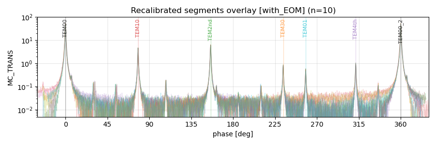
After the EOM installation, a representative post-EOM scan was taken with the same scan settings. For this measurement, the IMC transmission whitening gain was set to 30 dB. Unfortunately, the GPS start time for the post-EOM dataset was not logged at the time of measurement.
Notes
- The IMC is free-swinging during the scan; the JAC PZT signal is used as a proxy for the instantaneous laser frequency.
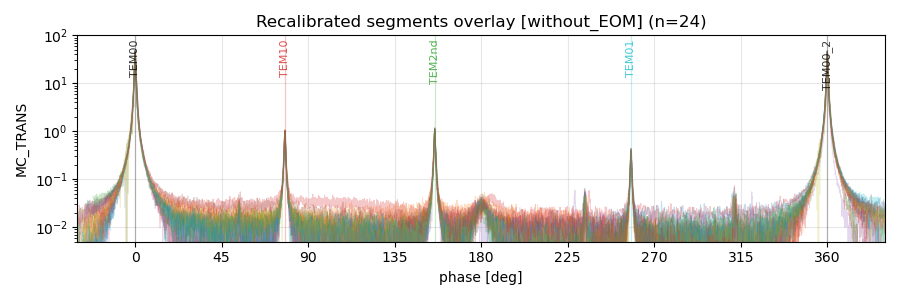
- Intentional yaw/pitch misalignment in the pre-EOM scans enhances TEM10/TEM01 as expected, confirming reliable mode identification and peak labeling.
- The IMC scan after the EOM installation exhibits noticeably stronger higher-order mode resonances than the pre-EOM reference scans.
- Calculation details can be found in the LIGO Git repo.
Result
- In the pre-EOM scans, the p-polarization resonance (π-shifted from s-pol) is visible at the \sim 0.1\% level, indicating a small but measurable mis-polarization component as shown in the second attached plot. The wider peak at the center is the p-pol resonance. The MC mirrors has higher transmissivity for p-pol the finesse for p-pol is lower than s-pol peaks.
- After the EOM installation, this p-polarization signature is no longer apparent, indicating that the mis-polarization is strongly reduced. It might be due to the filtering effect of the EOM. The mispolarized component caused by the input periscope is filtered by the EOM birefringence.
- In contrast, the post-EOM scan shows a substantially larger higher-order mode content (notably a large 2nd-order component ~10%), indicating significant mode mismatch in the current post-installation layout.
- A dedicated mode-matching calculation based on the as-built post-EOM layout will be reported separately in the near future.