Bottom line--If we collect fewer channels, that is, if the database has fewer Analog inputs to process, the database process time changes. This may seem obvious, but come on, we are collecting 15 pressure sensors, doing two or three calcs and the PID. Oh yeah, there is the 1 sec heartbeat, so sure, this processor is really stressed!
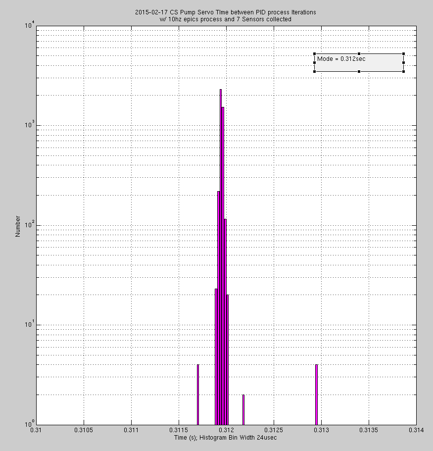
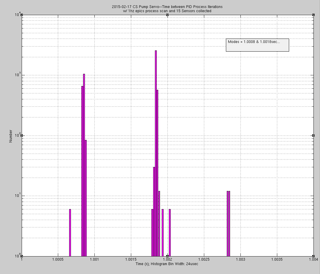
The first two attachments are matlab histograms of the DT field of the the epics PID. This is the time between the PID process iterations used in the PID calculation. In alog 16619 JeffK reports a DT value of 0.55sec; this is with 15 sensors collected and the epics running at 10 hz---the processor is only getting to the PID calculation every .55 sec! When I reduce the number of channels collected to 7, DT drops to 0.312 secs (first attachment.) In the second attachment is the histogram when the epics is set to run at a 1 second SCAN rate. Here, the PID record is processing at ~1second but is multimodal with about a 1mhz variation.
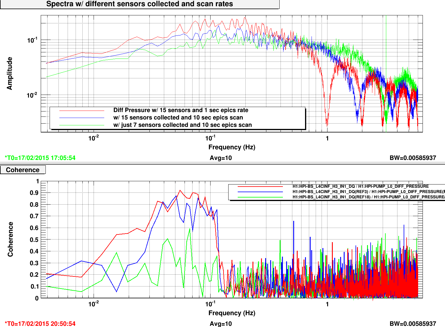
The third attachment is the Power Spectra of the Differntial Pressure running the Pump Servo and its coherence with the HEPI L4Cs at the BS. In the spectra you can see the zero related to the update period of the PID: Blue--15 sensors 10hz epics ==> 0.55sec update= 1.88hz; Red--7 sensors 10hz epics ==>0.312sec=3.2hz. And clearly Red: 15 chanels at 1hz ==> 1 sec update=1 hz.
The lower panel of the third plot shows the coherence with the Pressure to the BS HEPI L4Cs, it shows just H3 which had the strongest coherence in our normal configuration early Tuesday morning. The Blue Trace is that normal configuration of 15 sensors collected at a 10hz epics scan; the Green trace is when the sensors collected dropped to 7 as does our coherence with the reduced gain peaking. When we shift the process to 1hz scan shown in the Red trace (without adjusting the PID parameters!) the gain peaking increases as does our coherence again. As Jeff has done in alog 16782, we need to recalculate the PID parameters if we wish to reduce the epics scan rate.
A couple of comments / clarifications:
(1) I attach the extra bit of information -- we now have three different data points for these silly sods of CPUs:
Station  nSensors   CPU Clock Cycle
EX          6         0.288
Corner      7         0.312
Corner     15         0.552
A linear fit of these numbers reveals that we pick up 29 [ms] per sensor. Gross.

(2) Hugh's histograms of the clock-cycle were produced from ~5000 data points, querying the PID's subfield DT as he says. What's interesting is comparing the histograms from the three corner station data points,
7 Sensors     10 [Hz]   mostly-uni-modal, with a few slips -- 0.21% of the queries
15 Sensors    10 [Hz]   uni-modal
15 Sensors    1 [Hz]    tri-modal
where we're taken care to span the same clock cycle range, and to have the same bin-width in all histograms. Also note that when refiring to the time between modes in the 15 sensors, 1 [Hz] data, they're 1 [ms] (millisecond) apart, not 1 [mHz].
Interesting? Yes. Important? Probably not. If we're sampling at 1 [Hz], then a clock uncertainty at 1000 [Hz] should make very little difference to us.
It's more important that we can freely add and subtract sensors without having to worry whether the sampling rate will change, and/or be different than we request.

So, we'll stick with a 1 [Hz] requested sampling rate, and use the design from 16782 and confirm goodness.
