I analyzed the HWS data for the lock-acquisition that occurs around 1173641000. The "point source" lens appears very quickly (within the first 60s) and then we see a larger thermal blooming over the next few hundred seconds. I've plotted the data below (both gradient field and wavefront OPD). There are a few obviously errant spots in the HWS gradient field data. Since I'm still getting used to Python, I've not managed to successfully strip these off yet. However, it is safe to ignore them.
Check out the video too. Next step is to match a COMSOL model of thermal lensing with a point absorber to the data to get a best estimate of the size of absorber and the power absorbed (preliminary estimates are of the order of 10mW).
FYI: this measurement compares the system before, during and after a lock-acquisition (ignore the title that says "lock-loss"). The previous measurement, 34853, looked at lens decay before, during and after a lock-loss.
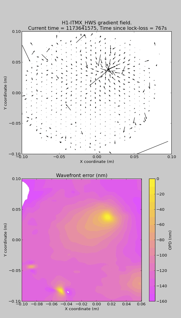

For your amusement I've attached a GIF file of the same data. My start time is 79 seconds prior to Aidan's "current time".
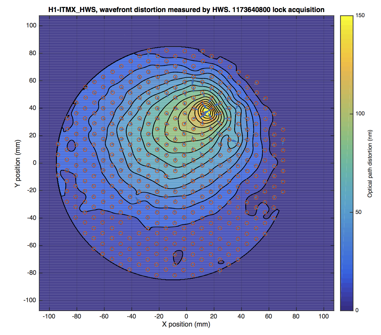
The integrated gradient field data for H1ITMX is contained in the attached MAT file. It shows the accumulated optical path distortion (OPD) after 2.75 hours following the lock acquisition around 1173640800. This is the total accumulated OPD for a round trip through the CP+ITMX substrates, reflection off ITMX_HR and back through ITMX+CP substrates.
- H1HWSX_wf_data.x = hswf.grid_x; % x coordinates of every point in WFcropped
- H1HWSX_wf_data.xUnits = 'm';
- H1HWSX_wf_data.y = hswf.grid_y; % y coordinates of every point in WFcropped
- H1HWSX_wf_data.yUnits = 'm';
- H1HWSX_wf_data.WFcropped = hswf.wf_numerical; % optical path distortion of every point in WFcropped
- H1HWSX_wf_data.WFcroppedUnits = 'm';
- H1HWSX_wf_data.t0 = 1173640800;
- H1HWSX_wf_data.t1 = 1173649900;
- H1HWSX_wf_data.deltat = 1173649900-1173640800;
- H1HWSX_wf_data.comments = 'Integrated HWS data. H1ITMX. Start (reference) and finish times are t0 and t1. x and y arrays contain coordinates. Cropped wavefront is central region where genuine data is believed to be. Outside the 85 mm radius is not real data'
Note: this image is inverted. In this coordinate system, the top of the ITM is at the bottom of the image.
Here is the wavefront data with the superimposed gradient field. The little feature around [+30mm, +20mm] does not appear in the animation of the wavefront or gradient field over much of the preceeding 2.75 hours. My suspicion is that this is a data point with a larger variance that the other HWS data points, rather than a true represtation of wavefront distortion.


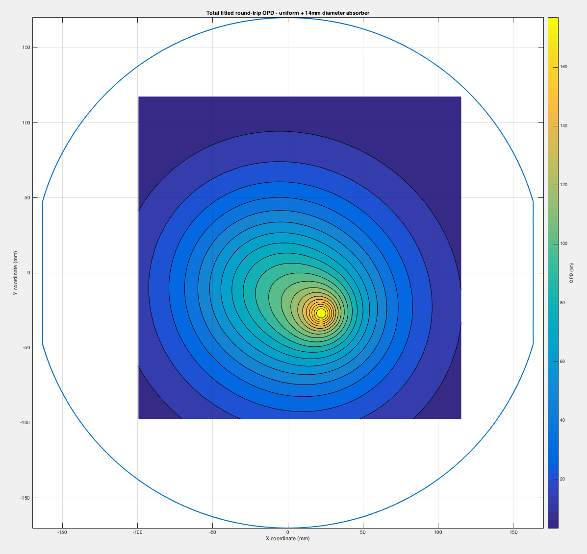
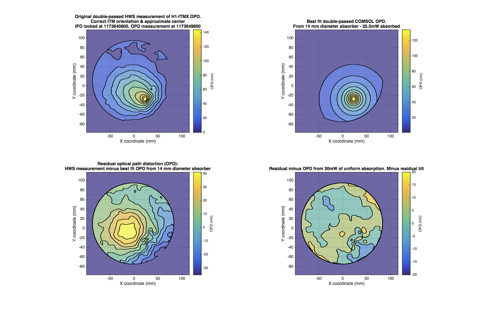
I fitted, by eye, a COMSOL model of an absorber (14mm diameter Gaussian, ~25mW absorbed) to the measured HWS data. I then removed this modeled optical path distortion to get the following residual (lower left plot). I then fitted a COMOSL model of 30mW uniform absorption to this model and subtracted it to get the residual in the lower right plot.
Here's the total fitted distortion from the sum of two COMSOL models (point absorber + uniform absorption):