Ansel Neunzert, Evan Goetz, Alan Knee, Tyra Collier, Autumn Marceau

Background

(1) We have seen some calibration line + violin mode mixing in previous observing runs. (T2100200)

(2) During the construction of the O4a lines list, it was identified (by eye) that a handful of lines correspond to intermodulation products of violin modes with permanent calibration lines. (T2400204) It was possible to identify this because the lines appeared in noticeable quadruplets with spacings identical to those of the low-frequency permanent calibration lines.

(3) In July/August 2023, six temporary calibration lines were turned on for a two-week test. We found that this created many additional low-frequency lines, which were intermodulation products of the temporary lines with each other and with permanent calibration lines. As a result, the temporary lines were turned off. (71964)

(4) It’s been previously observed that rung-up violin modes correlate with widespread line contamination nearby the violin modes, to an extent that has not been seen in previous observing runs. The causes are not understood. (71501, 79579)

(5) We’ve been developing code which groups lines by similarities in their time evolution. (code location) This allows us to more quickly find groups of lines that may be related, even when they do not form evenly-spaced combs.

Starting point: clustering observations

All lines on the O4a lists (including unvetted lines, for which we have no current explanations) were clustered according to their O4a histories. The full results can be found here This discussion focuses on two exceptional clusters in the results. The clusters are given here by their IDs (433 and 415, arbitrary tags).

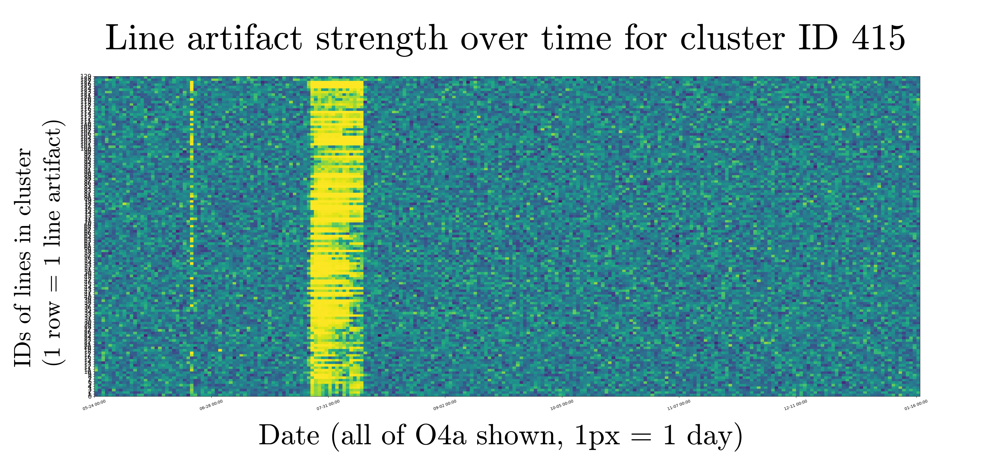
Cluster ID 415 was the most striking. It’s very clear from figure 1 that it corresponds to the time periods when the temporary calibration lines were on, and indeed it contains many of the known intermodulation products. However, it also contains many lines that were not previously associated with the calibration line test.

Cluster ID 433 has the same start date at cluster 415, but its end date is much less defined, and apparently earlier.

Given the background described above, we were immediately suspicious that the lines in the clusters could be explained as intermodulation products of the temporary calibration lines with rung-up violin modes. We suspected that the “sharper" first cluster was composed of stronger lines, and the second cluster of weaker lines. If the violin mode(s) responsible decreased in strength over the time period when the temporary calibration lines were present, the intermodulation products would also decrease. Those which started out weak would disappear into the noise before the end of the test, explaining the second cluster’s “soft" end.

Looking more closely - can we be sure this is violin modes + calibration lines?

We wanted to know which violin mode frequencies could explain the observed line frequencies. To do this, we had to work backward from the observed frequencies to try to locate the violin mode peaks that would best explain the lines. It’s a bit of a pain; here’s some example code. (Note: the violin modes don’t show up on the clustering results directly, unfortunately. Their positions on the lines list aren’t precise enough; they’re treated as broad features while here we need to know precise peak locations. Also, because the line height tracking draws from lalsuite spec_avg_long which uses the number of standard deviations above the running mean, that tends to hide broader features.)

As an example, I’ll focus here on the second violin mode harmonic region (around 1000 Hz), where the most likely related violin mode was identified by this method as 1008.693333 Hz.

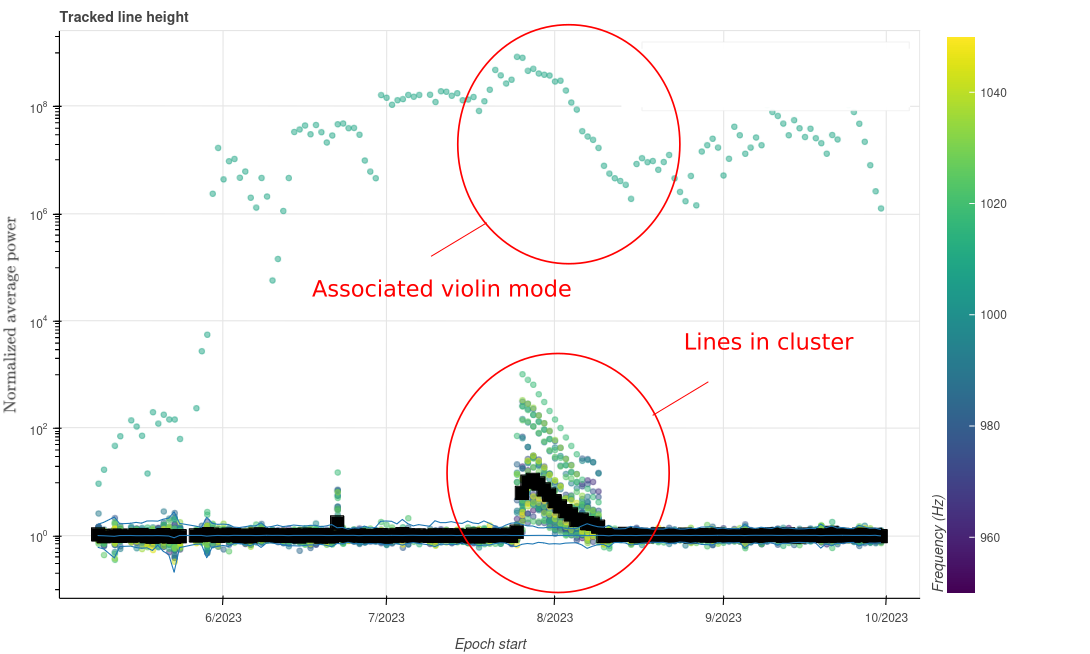
Figure 2 shows a more detailed plot of the time evolution of lines in the “sharper" cluster, along with the associated violin mode peak. Figure 4 shows a more detailed plot of the time evolution of lines in the “softer" cluster, along with the same violin mode peak. These plots support the hypothesis that (a) the clustered peaks do evolve with the violin mode peak in question, and (b) the fact that they were split into two clusters is in fact because the “softer" cluster contains weaker lines, which become indistinguishable from the rest of the noise before the end of the test.

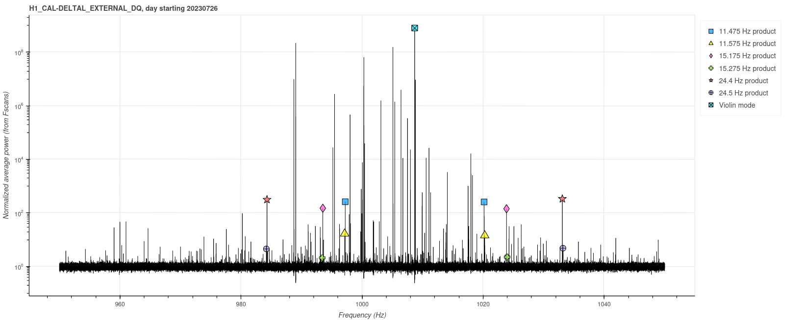
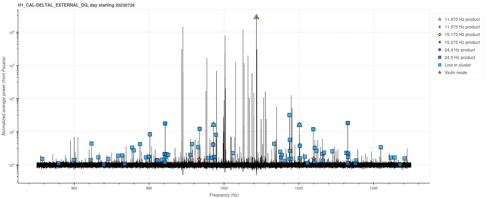
Figures 5 and 6 show a representative daily spectrum during the contaminated time, and highlight the lines in question. Figure 5 shows the first-order products of the associated violin mode and the temporary calibration lines. Figure 6 overlays that data with a combination of all the lines in both clusters. Many of these other cluster lines are identifiable (using the linked code) as likely higher order intermodulation products.

Take away points

Calibration lines and violin modes can intermix to create a lot of line contamination. This is especially a problem when violin modes are high amplitude. The intermodulation products can be difficult to spot without detailed analysis, even when they’re strong, because it’s hard to associate groups of lines and calculate the required products. Reiterating a point from 79579, this should inspire a caution when considering adding calibration lines.

However, we still don’t know exactly how much of the violin mode region line contamination observed in O4 can be explained specifically using violin modes + calibration lines. This study lends weight to the idea that it could be a significant fraction. But preliminary analysis of other contaminated time periods by the same methods doesn’t produce such clear results; this is a special case where we can see the calibration line effects clearly. This will require more work to understand.