This work was completed with help from Sheila Dwyer, Derek Davis, and Vicky Xu.
Sheila and Oli took 3000 seconds of no squeezing data on June 25 which I have used to run a correlated noise budget. This alog is long, but it details my methods to take this measurement while accounting for glitches, excess jitter noise and unsubtracted noise. I then discuss generating a noise budget using this data, and investigate the thermal noise level. There are many great background references for how the correlated noise is measured, but one of my favorites is Martynov et al. (2017).
I used the OMC DCPD A and B channels at 16 kHz, so this alog focuses on the correlated noise up to 5 kHz. Sheila is currently working on correlated noise measurements at higher frequency using the full-rate DCPD channels.
Executive summary:
These results show that above 1 kHz, the correlated noise is well-estimated by jitter noise from 1-2 kHz and our current frequency noise projection from 2-4 kHz. Above 4 kHz it appears we are overestimating the frequency noise, something that we could improve with a model of the CARM loop. Above 2 kHz, the frequency noise level is roughly a factor of 6-7 below DARM in amplitude. Jitter peaks are within a factor of 2-3 in amplitude from 1-2 kHz. The classical noise floor from 100-300 Hz appears similar to coating thermal noise with an amplitude that is 35% higher than our noise budget estimates. Below 100 Hz, we have not fully estimated our classical noise in the budget.
Jitter subtraction:
From 100-1000 Hz, I was able to use a strong jitter injection to estimate a transfer function and subtract the jitter noise from OMC DCPD A and B using IMC WFS A yaw as a single witness. The subtraction performed fairly well, with the exception that it injected a large peak just above 300 Hz where the jitter noise injection coherence dropped. I was also unable to get a strong enough measurement of the jitter coupling above 1 kHz so two broad jitter peaks remain in the data from 1-2 Hz. I applied a 1 kHz low pass to the subtraction to ensure that I only subtracted in the region with a high-fidelity measurement of the jitter transfer function.
Calculating the correlated noise:
I used a function written by Sheila and Vicky that applies the DARM OLG and sensing function using pydarm and the calibration model. The DARM OLG is applied to the correlated noise calculation using a formula written by Kiwamu Izumi in T1700131, equation 10. The resulting noise is calibrated into meters using the sensing function. I applied this correlated noise estimation method to the DCPD signals with and without jitter subtraction.
Managing bias from glitches:
Since the correlated noise budget requires taking a long data set, it is likely that the data will capture glitches which can bias the PSD and CSD estimates for the calculation, and possibly inflate the noise estimate. There are several methods that can be used to overcome this bias (gating, median averaging, etc). First, I found it useful to plot a whitened timeseries of each DCPD using the gwpy whitening function. This made it evident that there was one large glitch about halfway through the dataset. The gwpy gating function identified a 2 second period over which to gate. However, since the gating period was of a similar length to my fft length, I ended up choosing to reject the fft segments that included the glitch completely. I took a mean average of the remaining fft segments for the PSD and CSD estimates. Note that my method includes no overlap, which loses some resolution, but makes this calculation easier.
Accounting for unsubtracted incoherent noise:
For 3000 seconds of data, an fft length of 2 seconds, and two rejected PSD segments, the total number of averages is 1498. The largest possible amount of noise reduction in this method is sqrt(sqrt(1498)) = 6.2. This is sufficient to resolve the classical noise below 1 kHz, but not above. There are a few ways to improve the resolution for a fixed length. One is to reduce the fft length further to increase averages, since less frequency resolution is required at high frequency anyway (this is only useful if you don't care about your low frequency resolution). This plot shows a test of that, using different fft lengths for the same data length, with incoherent noise reduction ranging from a factor of 4.1 (fft length 10 s) to 8.8 (fft length 0.5 s).
You can also compare the correlated noise of the DCPDs (XCOR) with the noise in DCPD sum (SUM). The difference between these two noise estimates is the reduction of the incoherent noise (n), achieved in the correlated noise by the known factor of the number of averages (N). In other words, both noise estimates contain the same amount of classical noise (c).
SUM = c + n
XCOR = c + n/sqrt(N)
c = (XCOR - SUM/sqrt(N)) / (1 - 1/sqrt(N))
Without sacrificing the frequency resolution below 1 kHz, we can measure the classical noise above 1 kHz by accounting for any un-reduced incoherent noise. I compare a correlated noise estimate using this formula with my shortest fft length from above. For the rest of this post, I refer to this as the "full classical noise estimate"
Therefore, this work includes three different estimates of the correlated noise, one without jitter subtraction, one with jitter subtraction from 100-1000 Hz, and one with jitter subtraction and the application of my equation above. This plot compares these estimates with the unsqueezed DARM (aka SUM). All of these estimates use what I am referring to as the "excised mean average", which is the process I detailed above of excising ffts with glitches and mean-averaging the remainder.
Creating the noise budget:
I then added some of our noise budget traces: thermal noise, laser noise (frequency and intensity), controls noise (ASC and LSC), residual gas noise, and a correlated quantum noise trace generated using SQZ parameters from Sept 2024 (some likely out of date). Comparing these traces, it is evident that we have a large gap between our full classical noise estimate and our estimate of our known noises. First noise budget plot here
Evan Hall and Kevin Kuns did a similar exercise using pre-O4 data, alog 68482, and calculated that the thermal noise is approximately 30% higher than our estimate. I find a similar result using the jitter-subtracted correlated noise- the noise level from 100-300 Hz matches well with a thermal noise that is about 35% higher than our noise budget estimate, here is a ratio of the full classical noise estimate with the CTN estimate. I also find that the noise in this region is fairly gaussian. For example, I plotted the distribution of the ffts of the jitter-subtracted correlated noise at 105 Hz and their distribution matches a chi-squared distribution with two degrees of freedom (of course, this ignores the two outlier fft segments that contain the glitch). I referenced Craig Cahillane's dissertation appendix D: the PSD sample mean for gaussian noise with n samples follows a chi-squared distribution of 2n degrees of freedom. This should at least help convince us that the noise level here isn't being biased by some non-gaussian source; this was a concern that Vicky and I had when generating the correlated noise budget in the O4 detector paper.
I also recreated the noise budget with the thermal noise trace inflated by 35% here. Except for some unsubtracted jitter noise that I did not include in the budget, this effectively reconciles the correlated noise budget above 100 Hz.
These results show that we have also underestimated the noise below 100 Hz. It is not clear to me yet how much of that noise can be explained with a better estimate of the correlated quantum noise. Sheila and I are hoping to use some of the parameters she is generating from her sqz modeling to calculate possible lower and upper bounds of the correlated quantum noise and compare them with the entire correlated noise budget.

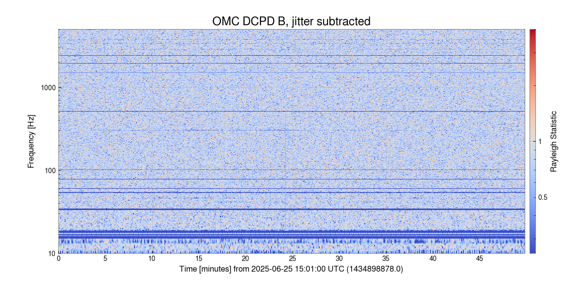
As another follow up on the gaussianity of the data, I made a spectrogram of the rayleigh statistic of each DCPD signal. Based on my (relatively new) understanding of the rayleigh statistic, I believe these plots are indicating that the DCPD data is fairly gaussian in the broadband, with one large glitch about halfway through the data set. This is the glitch that I discuss excising above.

And here is a text file that contains the frequency vector and correlated noise ASD (the red trace in this plot) in units of strain.

I am adding a comment to clarify that the thermal noise budget uses a Ti:Ta loss angle of 3.89e-4 rad, in line with the Gras 2020 paper, to calculate the coating thermal noise. My 35% increase estimate is therefore 1.35 * 1.13e-20 m/rtHz (at 100 Hz) = 1.52e-20 m/rtHz (at 100 Hz).
The O4 detector paper includes a full demonstration of the thermal noise budget, where the thermal noise is dominated by coating brownian noise, which is determined partially by the Ti:Ta loss angle. Therefore, I am assuming that if the overall thermal noise is higher by 35%, it is because the coating thermal noise is higher by 35%. I didn't make any fit of the slope, but the ratio of the noise with the thermal noise trace is fairly flat from 100-300 Hz.