matthew.evans@LIGO.ORG - posted 13:23, Sunday 11 September 2016 (29602)
PI damping model update (h1susprocpi, work permit 6149)
Matt, Terra (in spirit)
I have updated the h1susprocpi model to fix a few minor problems.
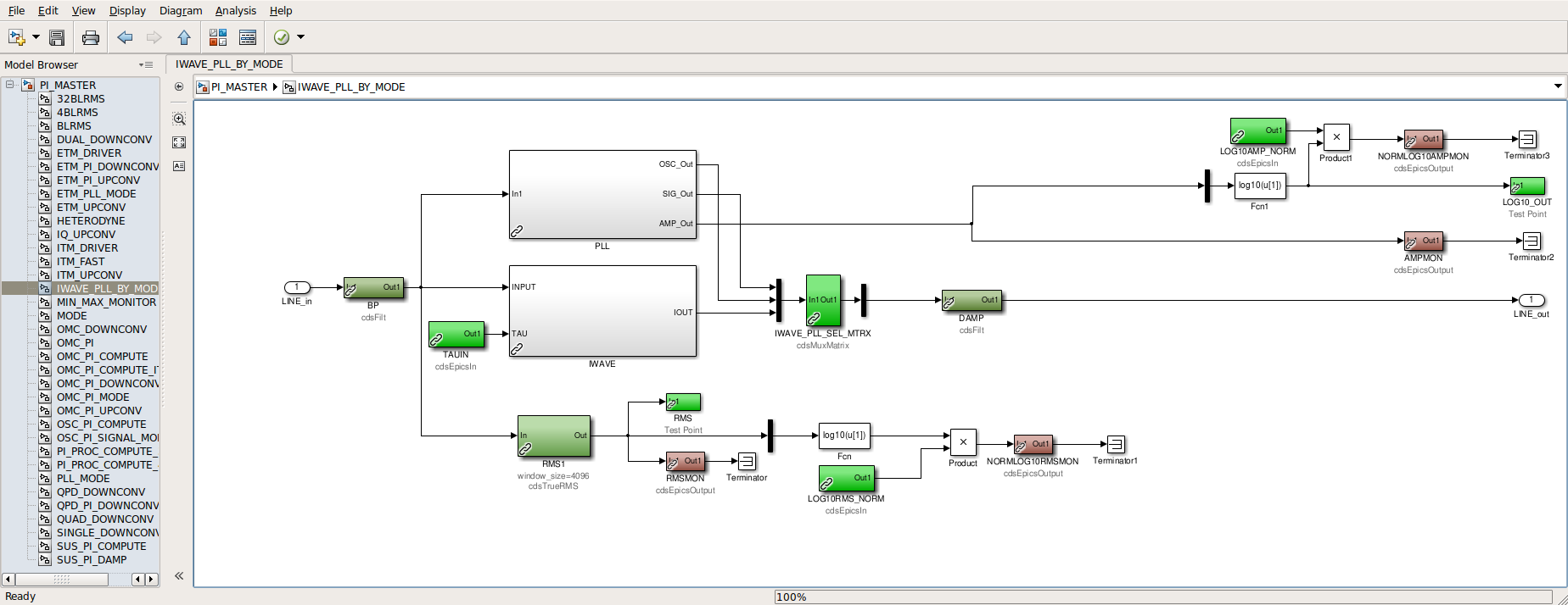
- the RMSMON was at the IWAVE output, which can be misleading, so I moved it to the BP output (see first image)
- the PLL phase was in the PLL loop, but the only real impact of changing the phase was to rotate the output phase (SIG_OUT) relative to the input signal. In-loop phase rotation can disturb the loop, so I moved the phase to the output. This will allow for quick phase adjustment even with a low UGF PLL. (It also flips the sign of the phase change relative to before, but the phase values are not set yet so this shouldn't matter.) The PLL screen should be updated to reflect this!
- OSC_OUT should now have an amplitude of 1, as should SIG_OUT when the amplitude scaling is unity. The amplitude was 2 before, so this simply divides both outputs by 2.
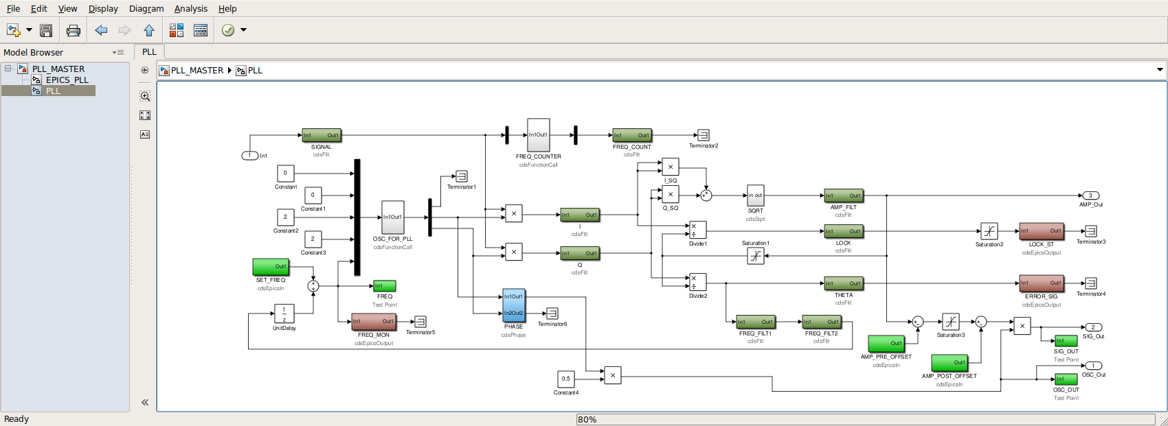
- changed amplitude scaling maximum from 1 to 10 ("Saturation3" in the second image). This will allow for lower gain settings in the PI DAMP filters, which gives smaller signals when the PLL is not locked and makes the gains more similar to the ones used for direct BP damping (usually 1k to 10k). Damping gains should not be greater than 10k, since an input of magnitude 10 will give 100k, which is close to DAC saturation.
-
added amplitude scaling offsets before and after amplitude scaling saturation (AMP_PRE_OFFSET and AMP_POST_OFFSET around "Saturation3", see second image).
- The reason for the PRE offset to is allow the output gain to go to zero (to inject little noise), even though the output of AMP_FILT is positive definite. (Generally, the PLL_SIGNAL_GAIN should be set so that the noise driven AMP_FILT_OUT is about 0.1.) Since this offset should always reduce AMP, it is subtracted from AMP (i.e., the value should be about +0.1).
- The POST offset is there in case we want to make an Amplitude Lock Loop (ALL) which keeps the input signal just about the noise floor so that the PLL can stay locked and track the mode. A small POST offset (also subtracted from the gain) will allow the gain to go negative for small values of the amplitude, thereby driving up the mode. This has not been carefully thought out, but it seems like it should give a stable ALL which just keeps the modes above the noise. The POST offset should be in the rage 0.0 to 0.1.
In terms of channel names, the impact of this model change should only be the addition of AMP_PRE_OFFSET and AMP_POST_OFFSET. I have only updated the models (i.e., I have not rebuilt the FE code, etc.). The corresponding work permit is 6149, and this change should go in with the next DAQ restart, or on Tuesday (which ever comes first).
Images attached to this report