Summary
A lower-estimate of absorption in the end test masses was measured using the end-station HWS cameras. This can be used to get a lower estimate of absorption in the test masses. I only got 30mins of data with the interferometer locked at 3W, we should repeat this measurement for a longer lock stretch to get a better idea of the absorption in the end test masses. The current measurement gives an absorption of 230ppb in ETMY and 130ppb in ETMX. Becasue we only measured for a 35min lock stretch, this will be an underestimate of the true test mass absorption. Also, the ETMY HWS measurement looks untrustworthy, so it would be worth checking the PZT off sets.
Details
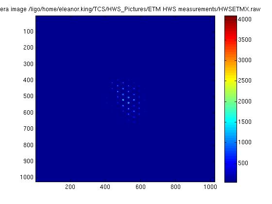
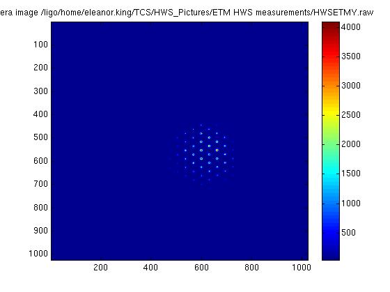
The EMT HWS cameras use the green als beam to measure the curvature change of the ETMs. We want a single reflection of the green beam off of the ETM, we cannot take this measurement when the green beam is resonant in the arm cavity. The green beam is usually shuttered and not present in the interferometer once the interferometer has reache DC_READOUT. To take a measurement with the HWS, once the interferometer is at DC_READOUT and the green beam is shuttered and no longer used, we re-open the ALS shutters and mislalign the green PZTs enough that the HWS sees no return beam from the ITM, only seeing a single bounce off of the ETM. I choose the PZT misalignment offsets as stated in alog 17860. Pictures of the HWS camera images are attached. Both cameras measure 22 centroids. The X-end image does not show a nice round beam, I may have to adjust the PZT alignment offset settings for this arm.
HWS reference centroids were taken before any locking started, with green PZTs in same misaligned state as we use when taking a measurement.
The ALS X/Y PZT2 are misaligned with type 'fixed', and with misalignment offsets:
H1:ALS-X_PZT2_PIT_MISALIGN_BIAS=15500
H1:ALS-X_PZT2_YAW_MISALIGN_BIAS=8300
H1:ALS-Y_PZT2_PIT_MISALIGN_BIAS=16100
H1:ALS-Y_PZT2_YAW_MISALIGN_BIAS=12000
The change in the spherical power of ETMY was 30udopters and ETMX was 11udiopters over a 35 minute lock stretch at 25.3W input power. For a change in spherical power of 1udiopter, 1.06mW of power is absorbed, according to Aidan's model of the test mass absorption (LLO alog 14634). The input power was 1.7W into the IMC, assuming 0.88 IMC-Faraday throughput efficency, 45 recycling gain, 280 arm cavity gain, 50:50 splitting ratio at BS, then 25.3*0.88*45*.50*280=140.3kW stored in the arms. Absorbed power/stored arm power = optical absorption. (Arm cavity gain is calculated using G_arm=(t_ITM/(1-r_ITM*r_ETM)).^2, where r_ETM=sqrt(1-TETM-L) and L=120ppm=loss in the arm. ) The arm power can also be caclulated using the four ASC_TR QPDs, which agree with the calulation using IMC input power, the variation between the four QPDs puts the uncertainty of the arm power at 15%.
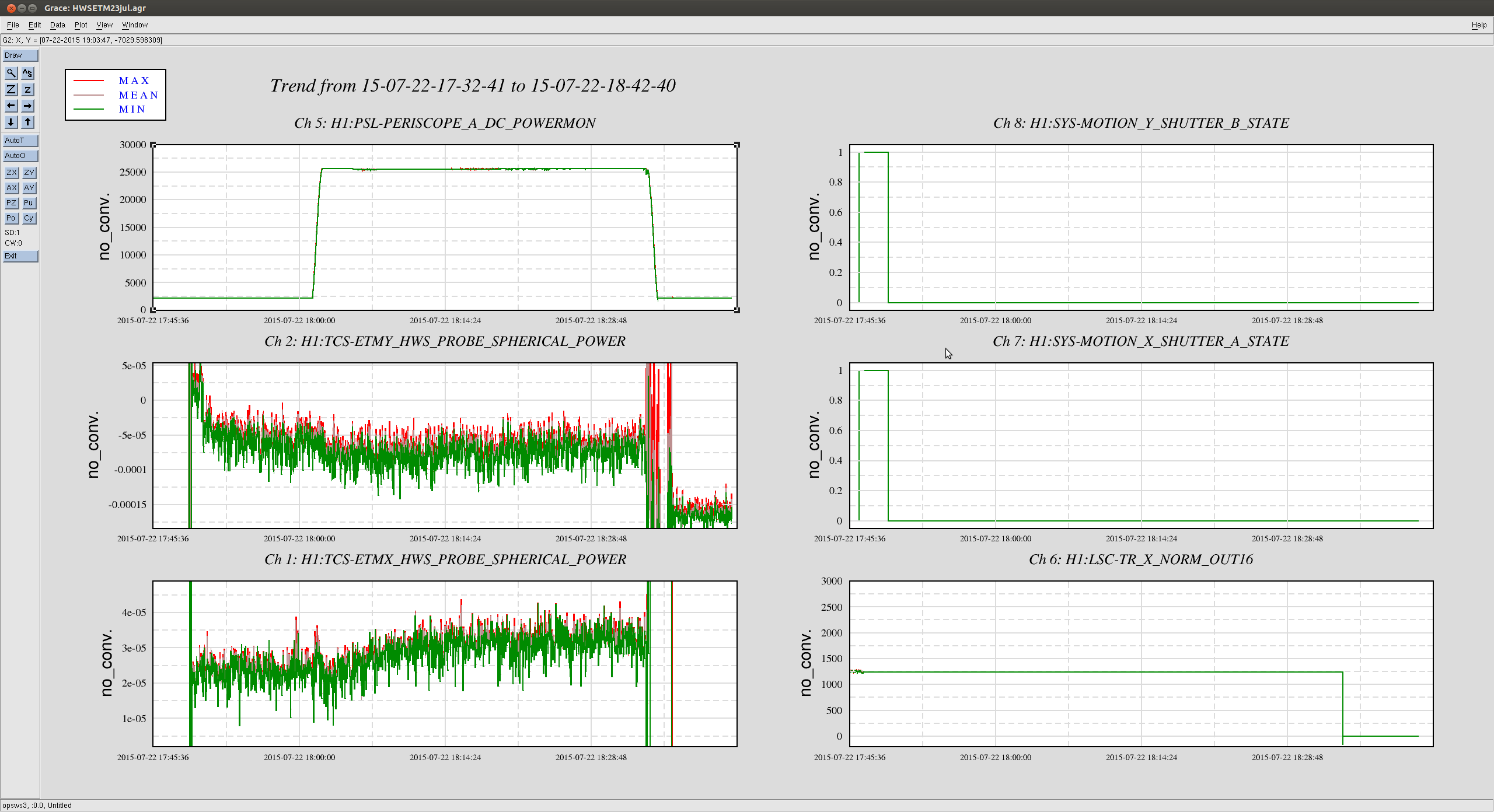
Attached is a dataviewer plot of the HWS spherical power output during a 30min lock at 25W. The shutters are opened when the shutter value=0. I have calculated an absorption value for both test masses, but the spherical power inn the ETMY is growing in the wrong direction. Either there is a sign error in a model or script somewhere, or this HWS is not set up correctly currently. I will investigate this.
|
|
ETMX |
ETMY |
|
spherical power at start of lock stretch at 23Jul 17:49:00 UTC(diopters) |
2.3e-5 |
-4e-5 |
|
spherical power at end of lock stretch at 23Jul 18:34:00 UTC (diopters) |
3.5e-5 |
-7e-5 |
|
change in spherical power (diopters) |
1.1e-5 |
-3.0e-5 |
|
absorbed power in test mass |
18mW |
32mW |
|
power in arm |
140.3kW |
140.3kW |
|
test-mass absorption (ppb) |
130ppb |
230ppb |
This measurement assumes the test masses have had enough time to reach thermal equilibrum, which actually takes longer than 30 mins. This means that the absorption measurement is an underestimate. It would be desirable to get a measurement of a lock stretch of >1hr. The HWS measurement itself is quite noisy.