[Rodica, Kiwamu, Dick, Michael R., Keita, Paul]
Last night and today we finally managed to get what looked like a good measurement of the IMC pole response. Here is a brief description of the measurement setup:
Swept sine signal applied directly from the SRS785 to the AOM driver box inside the PSL. Frequency range was 1kHz to 100kHz, signal amplitude was 400mV pkpk. 1000 intergration cycles, and 101.56ms integration time. Measurement was a transfer function from the DCPD on the PSL installed recently (PDA55) to the DCPD on the IOT2L table (DET100A). ~200mW injected to modecleaner.
The PDA55 on the PSL table didn't give us an observable signal from the amplitude modulation previously when we tried on Wednesday. Rodica checked the Thorlabs recommendation for best linear performance, which states that the maximum intensity should be less than 10mW/cm^2. Even with a very low beam power we may have been exceeding this value due to the very small beam size. The PD was therefore moved to have a larger incident beam size.
We were struggling to get a decent signal on the SRS785 until Kiwamu suggested reducing the light power reaching the PDs to less than 1V. Once we brought the power down to less than 600mV, we were able to see a decent signals on the SRS785 and began taking TFs.
The first attached transfer function is directly from the PSL PD to the IOT2L PD. In the event that the response of both PDs is linear, this should just give the cavity response. However, we noticed that the phase dropped below -90deg on the TF, indicating the presence of another pole - likely that of one of the PDs. We therefore took a TF from the PSL PD to the IOT2L PD, with the IOT2L PD repositioned in the IMC REFL path and the cavity misaligned (as Giacomo did previously). This TF is the second attached plot, and shows the pole of the IOT2L PD. Finally, we then divided the first transfer function by the second to eliminate the different PD response, leaving us just with the cavity response. This transfer function, along with a fit, is shown in the third attached plot.
For now, I just fitted the phase of the pole measurement, which gave the result 8812.36 Hz for the cavity pole. I'll try a complex data fitting routine soon and post the result.

Puzzled by the fact that my previous measurement of the cavity pole didn't make much sense, I spent some time playing with differnt fitting algorithm and writing a simple rountine to fit complex valued functions. It didn't help with my data (there's apparently something I'm missing in the response of some of the compoenents...), but I got a chance to fit this measurement.
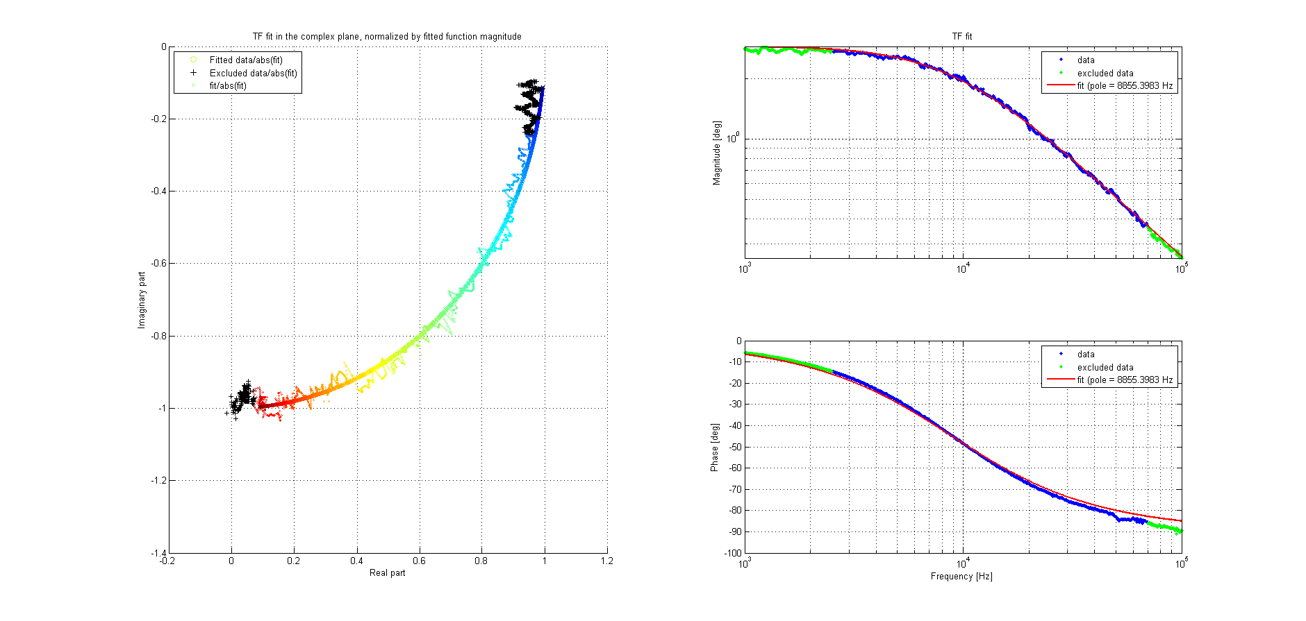
Of the attached figure, the two plots on the right don't need any explanation. The one on the left, intead, its a bit odd and needs some explanation (but I like it!). It is built by plotting the complex TF experimental data points and the LP filter fitting function both divided by the magnitude of the fitting function itself. The fitting parameters are obtained by minimizing the quantity:
abs( ( data(f) - fitfunt(f) ) / fitfunc(f) )^2
The reason for normalizing by the value of the fitted function is that, in this way, the points with very small magnitude have the same relative weight of the ones with large magnitude (analogous as fitting in dB scale with uniform weighting), that wouldn't be true otherwise. For the same reason I plotted the normalized quantitites instead of the normal ones, so it is easier to see how "relatively" far the fitting function is from the data, regardless fo their absolute magnitude.
The plot is actually a 3D plot seen from above (you can rotate it in the ".fig", obviously not in the ".png"), with the z axis being the log(frequency). log(frequency) also set the color of the points, so that when you look at the graph projected on a plane (i.e. from above) you can still somehow see the frequency dependence. If the fit is good, the fitted points and the measured ones should be close in both position on the plane AND color.
I excluded the points <2.5e3 Hz and >7e4 Hz from the plot for direct comparison with similar fits done at LLO. The result is definitely close to the expected cavity pole value (8.717 kHz), but I should point out that the choice of the fitting range could change this value by a couple hunderd Hz (for example it increases to about 8950 Hz if I include the entire range of data), so we should pay attention not to take this result to be more accurate that it actually is.