Craig, Sheila
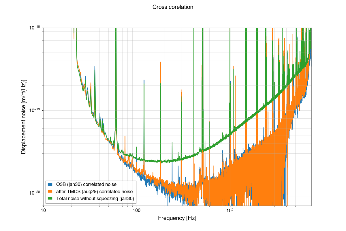
Attached is a plot of the cross correlated noise with the squeezer off taken on Aug 28th after the TMDS (56632) compared to an hour of data taken without the squeezer on because of difficulties on Jan 30th.
It has taken me a while to get this posted because I realized that in the cross correlation code I used previously I was using median averaged PSDs, and mean averaged CSDs. This plot was made incorportaing code from Craig that he has written to correctly do median averaging for CSDs (scipy has an error in the way it calculates a median averaged CSD). Craig is writting up in his thesis the correct way to do this calculation.
Both of these traces are made with 1 hour of data, although there is more data available for Aug 29th I could not find longer stretches without squeezing in O3. I had in the past relied on 10 minutes of data to get a rough cross correlation, but longer stretches of data are generally needed.

Attaching four plots of the LHO correlated noise, on top of what Sheila's done.
Also attaching four .txts of the data in the first plot, for comparison with the future.

Plot 1: Comparison of DARM noise and correlated noise ASDs from times in O3 with no squeezing (October 2019 vs August 2020).
For 2019 we have 20000 averages from 10000 seconds of data.  For 2020 we have 67156 averages from 33578 seconds of data.  This is why blue is more noisy than orange, and why these plots are less noisy than those in the original post.  These spectral densities use a binwidth of 2 Hz and no overlap.

The correlated noise from 1 kHz up is higher everywhere.  The noise above 3 kHz comes from laser intensity noise.  The noise between 1 kHz and 3 kHz is not understood, but it too is higher.

Plot 2: August 2020 correlated noise plot, with auxiliary traces.
This plot confirms the median-averaging and "PSD rejection" technique give the same result for the correlated noise, and shows the results of mean-averaging if no glitch-mitigation is performed.

"PSD rejection" is where large PSDs and CSDs are strategically thrown out of the analysis, in an effort to remove glitches in the analysis.
"PSD rejection" works by throwing out PSDs with values higher than 14 times the median at a single frequency (I chose f = 40 Hz).
Purely statistically, this should accept 99.9938% of the PSDs, or reject only 4 of 67156 of the averages.
In reality, 53 PSDs are rejected and eliminated from the mean-averaging, meaning this method has eliminated about 49 glitches from the analysis.
When a PSD is rejected, the associated CSD is rejected as well.
"PSD rejection" is less difficult than median-averaging, but throws out PSDs and CSDs somewhat arbitrarily.
At such a high cutoff, this should not affect our analysis significantly.

Plot 3: Coherence and CSD median-bias calculation.
It is commonly known that a median-averaged PSD has a mean-to-median bias of log(2) for large number of averages.  To recover the mean-averaged PSD, the median-averaged PSD must be divided by log(2).
The case is the same for median-averaged CSDs.  The difference is the bias varies between log(2) down to 1/2, depending on the coherence of the signal.
We can use the median-averaged coherence to estimate (numerically) the CSD mean-to-median bias.
The results are shown here.
The derivation of the bias is in my thesis, Figure A.9 an A.10.

Plot 4: 2D histogram of all 67156 correlated noise CSDs at f = 700 Hz, with 1D histogram projections.
This plot illustrates what we are looking for when estimating small correlated noise within signals with high uncorrelated (shot) noise.
Random shot noise has a random phase, and so the mean and median of the shot noise should average away to zero with a 2D Laplace distribution.
The correlated noise always has the same phase, and should eventually stack and rise out of the noisy floor.
This skews the resulting distribution into an asymmetric Laplace, with a skew factor kappa.
This correlated noise is where the CSD will average to given infinite samples.
Usually we represent this correlated noise as an ASD = sqrt(abs(CSD)), as in Plots 1 and 2.

