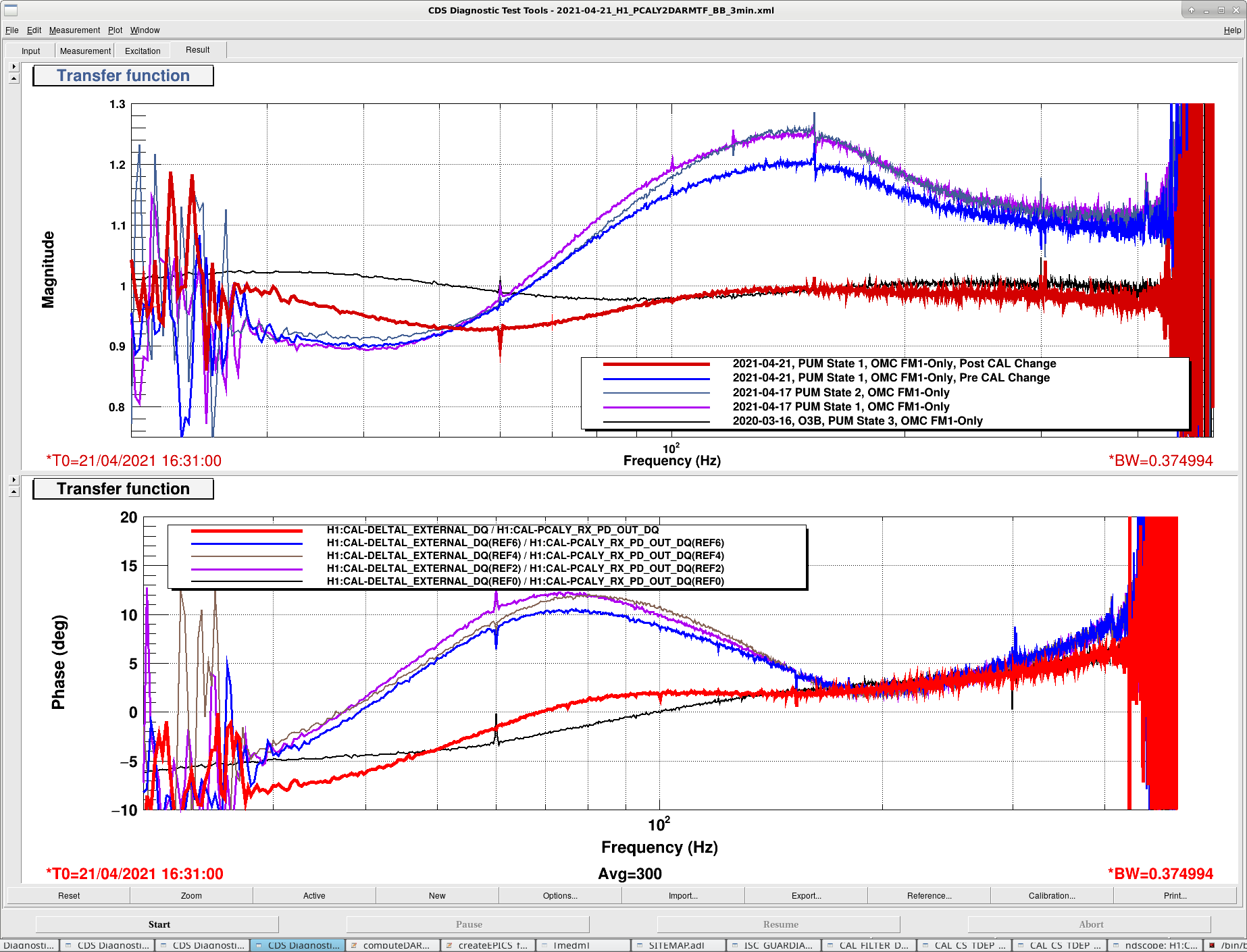
J. Kissel

Using the measurements and fit zeros and poles from LHO:61313, I've now created a compensation plan for the PUM driver recently modified a la E2100204. We are armed with all the right z:ps to compensate the newly modified ETMX PUM driver in the front-end, and most importantly we know quantitatively how much systematic error in the DARM loop calibration the residual response will incur. 

The plan: compensate all the sub-nyquist poles and zeros in the front-end, and suggest that -- pending discussion of how complicated it will be with the pyDARM / GDS / DCS team -- we compensate the super-Nyquist poles in the low-latency and offline calibration pipelines.

In the main portion of the aLOG, I'm going to focus on State 3 -- the lowest noise, "Low Pass ON," state, that we intend and hope to operate in. I also have a plan and plots to equally well compensate State 1 (no switchable response on) and State 2 (highest range, high gain, "Acquire ON" state), and will do so, but it distracts from the methods and conclusions for State 3, so I'll add comments later. (The plan for State 4, the awkward, rarely-used, LP ON and ACQ ON state that is somewhere in between State 1 and State 3 in response comes "for free" with the compensation plan for the other three states, since it's a linear combination of State 2 and State 3). 

I tell the story with the collection of plots attached.
(1) 2022-01-14_H1SUSETMX_PUMDriver_S1000343_40Ohm_AllStateModels_UL.pdf 
Here, for one coil, I just show you a reminder of the expected response of each state -- using the UL coil as the demonstrative example. Remember, roughly, we expect from the design that

                Zeros (Hz): Poles (Hz)
    State 1            [12] : [110]
    State 2          [1.35] : [80]
    State 3   [12, 25, 110] : [2.5, 110, 1200]   # a combination of State 1's 12:110, and the newly redesigned z:p response of LP filter

but when we consider the coil driver & AOSEM system response, we also need to add a [z] = 850 Hz. This plot shows the magnitude and phase of the *measured* data in solid lines, which is 
    coil driver & AOSEM system response = coil driver response in each state (with 40 Ohm load) 
                                          * AOSEM response (from the ratio of State 1 under the two different loads).
and the corresponding (normalized) fit response in dashed lines. Of course, on a loglog plot that spans 6 orders of magnitude, everything looks excellent. So, let's zoom in.

(2) 2022-01-14_H1SUSETMX_PUMDriver_S1000343_40Ohm_State3_AllCoilsCompensationComparsion.pdf
In this collection of 4 plots for 4 coils, in each I show the following comparison for State 3,
    (BLUE) The the measured data (again, coil driver TF * AOSEM TF), normalized the unity by dividing out the magnitude of the measured data at the lowest frequency point, 0.2 Hz. 
against the following three compensation possibilities,
    (ORANGE) If we, ideally, compensate for every single fit zero and pole, including the super-nyquist ~17.5 kHz zero in the AOSEM response.
    (GREEN) If we scrap the super-Nyquist 17.5 kHz AOSEM pole and only compensate with all low frequency z:ps. Note here, this does include all the "nearly canceling" zeros and poles, not just the expected ones near the z:p frequencies listed above.
    (RED) If we compensate only for the coil driver response, and incorrectly ignore the AOSEM response.
where in the left two panels are the magnitude and phase of each, and in the right two panels the magnitude and phase of the product of the two -- i.e. what will be leftover after compensation, i.e. the systematic error in the model for each coil -- which we model to have identically, and frequency independent, unity (1.0) magnitude and zero (0.0) phase.

One can see that if we ignore the AOSEM response, as we've done in the past, for each coil we incur a systematic error that's increasing rapidly with frequency, reaching 2.5% / 4 deg already by 100 Hz -- where the PUM actuator is still a big part of the DARM loop response. No thanks!

Speaking of, now's the part where I remind you of the relatively new, but incredibly instructive plot that shows what part of the DARM loop contributes systematic error to what frequency band.

(3) 2021-04-23_H1_PostO3_pydarm_modelparams_ResponseFunctionContributions.pdf
Using the new pyDARM "2.0" DARM Loop Model infrastructure and a newly crafted parameter set, pydarm_modelparams_PostO3_H1_20210423.ini, based on the older, "1.0" pyDARM parameter set used to calibrate the IFO during the Post O3, post ITMY swap to remove point absorber, IFO (see LHO aLOGs 58729, 58691, and 58656), I show the magnitude of the relative contributions to DARM of each major component of the DARM loop response function, R. Remember,
    h = (1/L_4karms) * R * d_err
    R = (1/C + [A_U + A_P + A_T]*D)

with h as the strain on the detector (our gravitational wave channel), d_err as the input error signal to the DARM filter bank (a digitized version of the DCPDs), C as the interferometric response of the arm cavity displacement to d_err, D is the DARM loop digital control filter turning d_err into a control signal d_ctrl that's sent out to the QUADs for actuation, and A_U, A_P, and A_T are the UIM (L1), PUM (L2), and TST (L3) QUAD actuator stage responses from request to displacement of the test mass (modeled as a single QUAD, regardless of whether, say A_U and A_P are ETMY, and A_T is ETMX). So, this plot shows the magnitude of each of the four terms, 1/C, A_U*D, A_P*D, and A_T*D divided by the overall response, R. For each trace, one reads the plot as "where the function lands as a function of frequency, is the relative contribution of that term to DARM. So, if there's (frequency-dependent) systematic error in that term, then that error gets amplified or suppressed by this function."

For out purposes here, we see that the PUM term, A_P*D/R, is a major contributor to the response function from the lowest frequency plotted (~0.1 Hz) all the way to 250 Hz, where its contribution drops below a factor of 0.01, or 1%. Importantly, that means -- right in the most sensitive regions of the detector, between ~20 and 200 Hz -- systematic error in the PUM stage is only suppressed by at most 10%, and gain peaking in the cross-overs between the sensing function ([1/C]/R), the test mass stage ([A_T*D]/R), and the UIM stage ([A_T*D]/R), all cause *amplificiation* of any systematic error in the PUM stage within the DARM loop response, by as much as a factor of ~1.5.

So, let's propagate the individual coil's systematic error -- the right-hand panels in (1) -- through A_P to the response function, R, in a two step process.

(4) 2022-01-14_H1SUSETMX_PUMDriver_S1000343_40Ohm_State3_etaPUM_Comparison.pdf
Here, I show the magnitude and phase modeled systematic error in the PUM actuation transfer function. This is done my taking the product of compensation * coil driver (& AOSEM) transfer function "residual" (i.e. the right panels of the plots in (1)) as a multiplicative factor, \eta_PUM to the model of A_P. For this, through the power of linear algebra, we don't even need A_P, since
    A_P = 0.25 * (A_P_UL + A_P_LL + A_P_UR + A_P_LR)

and we model the response from all coils to be ideally the same, A_P_UL = A_P_LL = A_P_UR = A_P_LR = A_P. And thus
    \eta_A_P = A_P (with sys error) / A_P (no sys error) 
               (0.25 * \eta_A_P_UL * A_P_UL + 0.25 * \eta_A_P_LL * A_P_LL + 0.25 * \eta_A_P_UR * A_P_UR + 0.25 * \eta_A_P_LR * A_P_LR)
             = -----------------------------------------------------------------------------------------------------------------------
                                         (A_P_UL + A_P_LL + A_P_UR + A_P_LR)
               0.25 (4 * A_P) (\eta_A_P_UL + \eta_A_P_LL + \eta_A_P_UR + \eta_A_P_LR)
               = --------------------------------------------------------------------
                                       0.25 (4 * A_P)
    \eta_A_P = 0.25 (\eta_A_P_UL + \eta_A_P_LL + \eta_A_P_UR + \eta_A_P_LR)

I hold the color scheme across the remaining plots, so again
    (ORANGE) Compensating for all z:ps, including super-Nyquist ps
    (GREEN) Compensating for all low-frequency z:ps, but dropping super-Nyquist ps.
    (RED) Compensating only for the coil driver response, and incorrectly ignore the AOSEM response.

We all agree that we want to compensate for the AOSEM response, so let's jump to the comparison of compensating only the sub-Nyqiust vs. compensating for for it all. Compensating only the sub-Nyquist, former, "redux," collection of z:ps, alone actually yields pretty awesome results --  below 0.1% / 0.5 deg error below 100 Hz. Nice! Maybe we can get away without adding the complexity of compensating for super-Nyquist z:ps.

But the proof is in the pudding -- this error propagated through (3) to show the error in the response function, R.

(5) 2022-01-14_H1SUSETMX_PUMDriver_S1000343_40Ohm_State3_etaR_w_etaPUM_Comparison.pdf
Here's the final answer of the model -- the estimated error in the PUM stage, propagated to error in the response function. That is, 
    \eta_R = R (with sys error in A_P) / R (no sys error)
             (1 + G (with error in A_P) ) / C) 
           = -------------------------------
             (1 + G (no error in A_P) ) / C) 

                 [[ G = A*D*C = [A_U + A_P + A_T]*D*C ]]

             1 + [A_U + \eta_A_P * A_P + A_T]*D*C
    \eta_R = ------------------------------------
                  1 + [A_U + A_P + A_T]*D*C


This plot is conclusive: 
    (i) RED We must compensate for the AOSEM response. I'm not sure how we've gotten away with not compensating for this response before. Typical *measurements* (not models or estimates, but PCAL \Delta L to the final product h measured transfer functions) of systematic error in O3 were at the level of the RED curve, so it adds a bit of distrust to my model. But, then I remember that there are *plenty* of systematic errors, in A_U, A_P, A_T, and (1/C) that are all co-mingling with various (and never shown) phases. So, it could be quite possible that we've been fortunate and had some canceling systematic errors in these terms. I *also* remember that in PostO3 times, even after updating the (1/C) to reflect the newly awesome, point-absorber-free interferometric response, we had 1.0 - ~8% level error between 10 and 100 Hz -- see 2021-04-21_PCAL_2_DELTALEXT_TF.png from LHO:58691. Note... that was measured with the PUM driver in State 1, which this aLOG doesn't focus on, and I'm not sure was ever well compensated... yeah... you get the point -- even if there's something fishy about the modelled results -- we need to compensate for the AOSEM response.

    (ii) GREEN If we ignore super-Nyquist poles from the AOSEM response, and we are OK with incurring a known, sharply featured, frequency-dependent error in the response function, that maxes out at "only" 0.3% / 0.2 deg at 100 Hz / 50 Hz, then we could save ourselves the person-power and complexity of adding in individual coil compensation in the low-latency / offline calibration pipelines. I'm on the fence about this one. We do already compensate for super-Nyquist poles on the test-mass stage actuator, so it would "only" be and "extension" of that, but in the new pyDARM 2.0 era, we sacrifice easy extensibility for modular, well-documented, unit-tested, perfect python code. I'll being the discussion to the greater team, and see what they decide.

    (iii) ORANGE If we compensate for all fit poles and zeros, we could essentially forever ignore any systematic error in the PUM driver. Response function systematic error from not modeling any electronics of the PUM driver would be at the 0.1% / 0.2 deg level. Wouldn't that be cool?

Anyways -- For now, we are armed with all the right z:ps to compensate the newly modified ETMX PUM driver in the front-end, and most importantly we know quantitatively how much error that will incur. 

Indeed, I have this for all three states of the ETMX PUM driver.

I plan on waiting until *after* all the front-end are rebooted tomorrow to do the install. (Feb 15, see fallout from 10232 and LHO:61673)