joseph.betzwieser@LIGO.ORG - posted 12:40, Friday 01 September 2023 - last comment - 12:11, Friday 17 November 2023(72622)
Calibration uncertainty estimate corrections
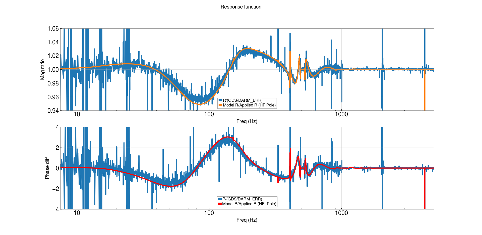
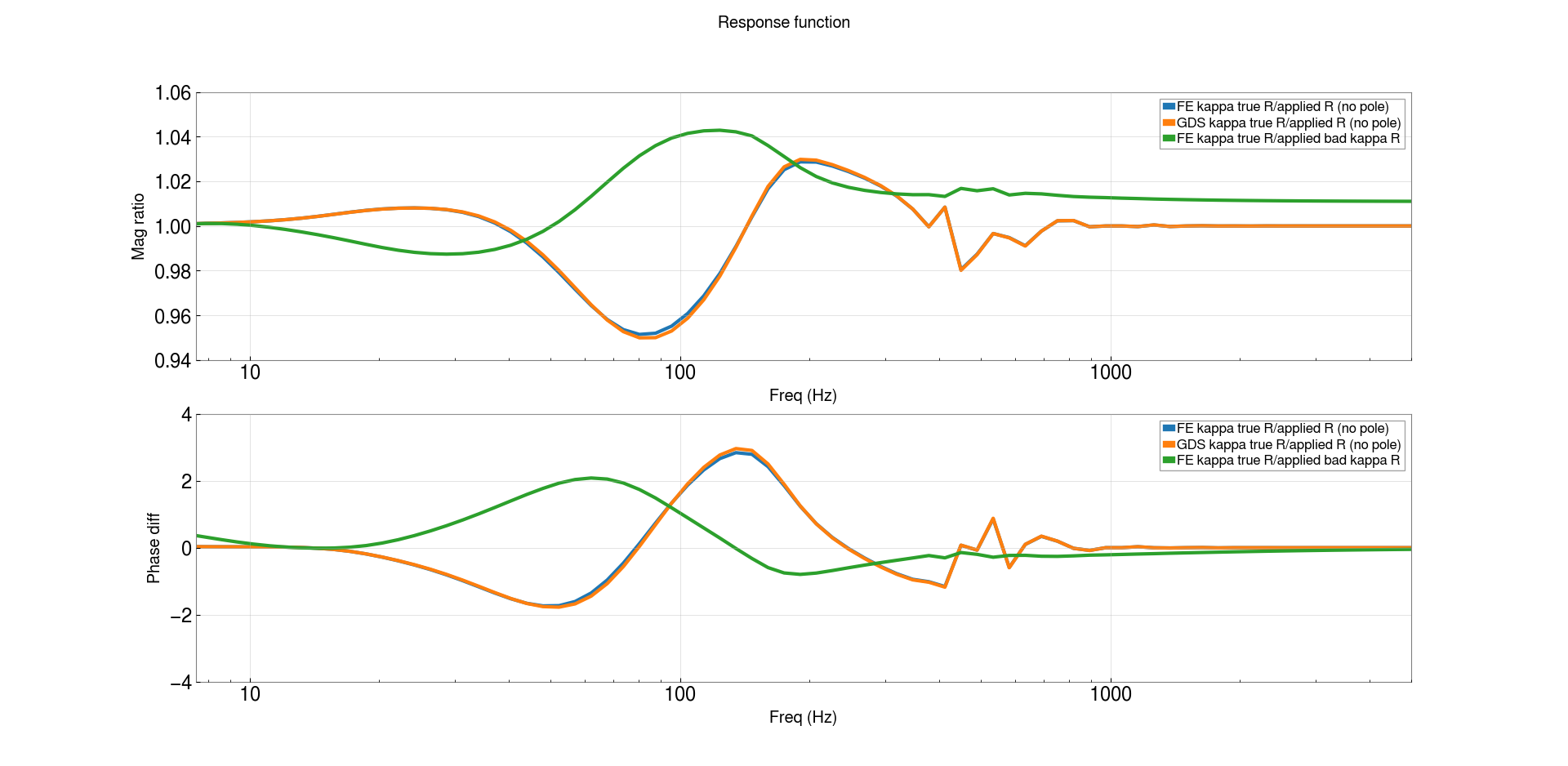
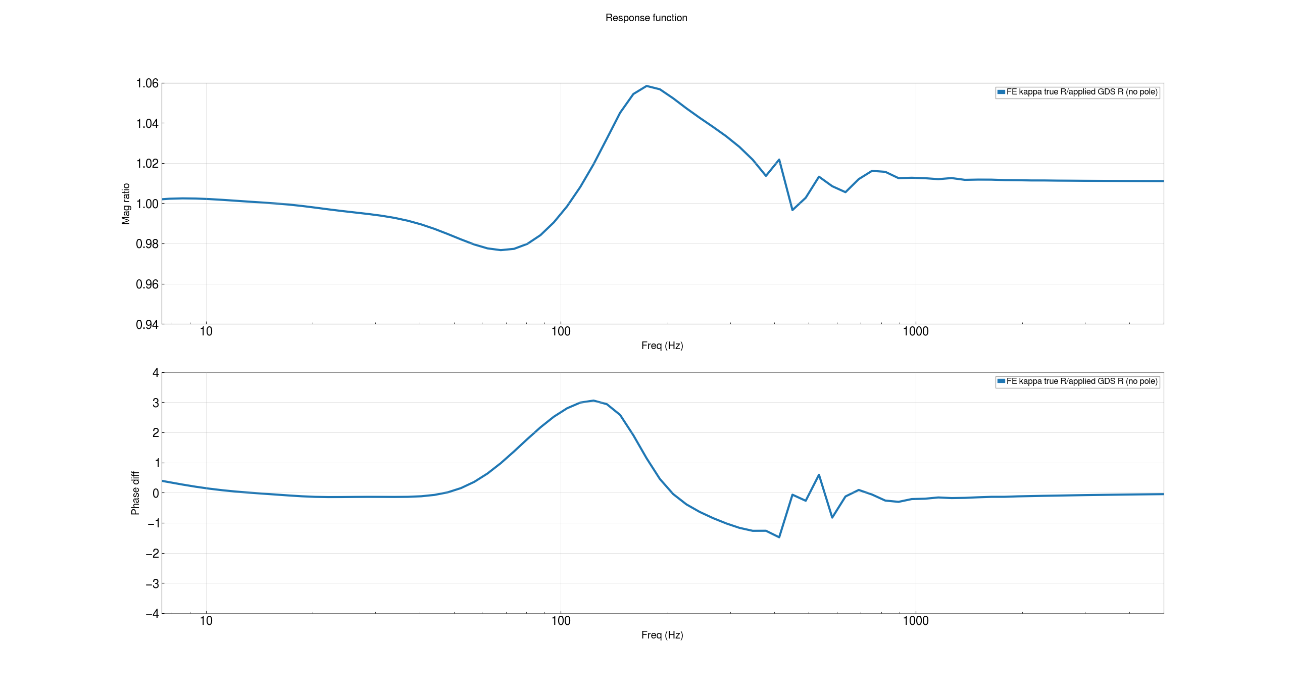
This is a continuation of a discussion of mis-application of the calibration model raised in LHO alog 71787, which was fixed on August 8th (LHO alog: 72043), and further issues with what time varying factors (kappas) were applied while the ETMX UIM calibration line coherence was bad (see LHO alog 71790, which was fixed on August 3rd.

We need to update the calibration uncertainty estimates with the combination of these two problems where they overlap.  The appropriate thing is to use the full DARM model (1/C + (A_uim + A_pum + A_tst) * D), where C is sensing, A_{uim,pum,tst} are the individual ETMX stage actuation transfer functions, and D is the digital darm filters.  Although, it looks like we can just get away with an approximation, which will make implimentation somewhat easier.

As a demonstration of this, first I confirm I can replicate the the 71787 result purely with models (no fitting).  I take the pydarm calibration model Response, R, and correct it for the time dependent correction factors (kappas) at the same time I took the GDS/DARM_ERR data, and then take the ratio with the same model except the 3.2 kHz ETMX L3 HFPoles removed (the correction Louis and Jeff eventually implemented).  This is the first attachment.

Next we calculate the expected error just from the wrong kappas being applied in the GDS pipeline due to poor UIM coherence.  For this initial look, I choose GPS time 1374369018 (2023-07-26 01:10), you can see the LHO summary page here, with the upper left plot showing the kappa_C discrepancy between GDS and front end.  So just this issue produces the second attachment.

We can then look at what the effects of the 3.2 kHz pole being missing for two possibilities, for the Front end kappas, and for the GDS bad kappas, and see the difference is pretty small compared to typical calibration uncertainties.  Here it's on the scale of a tenth of a percent at around 90 Hz.  I can also plot the model with the front end kappas (more correct at this time) over the model of the wrong GDS kappas, for a comparison in scale as well.  This is the 3rd plot.

This suggests to me the calibration group can just apply a single correction to the overall response function systematic error for the period where the 3.2 kHz HFPole filter was missing, and then in addition, for the period where the UIM uncertainty was preventing the kappa_C calculation from updating, apply an additional correction factor that is time dependent, just multiplying the two.

As an example, the 4th attachment shows what this would look like for the gps time 1374369018.
Images attached to this report
Comments related to this report
For further explanation of the impact of Frozen GDS TDCFs vs. Live CAL-CS Computed TDCFs on the response function systematic error, i.e. what Joe's saying with
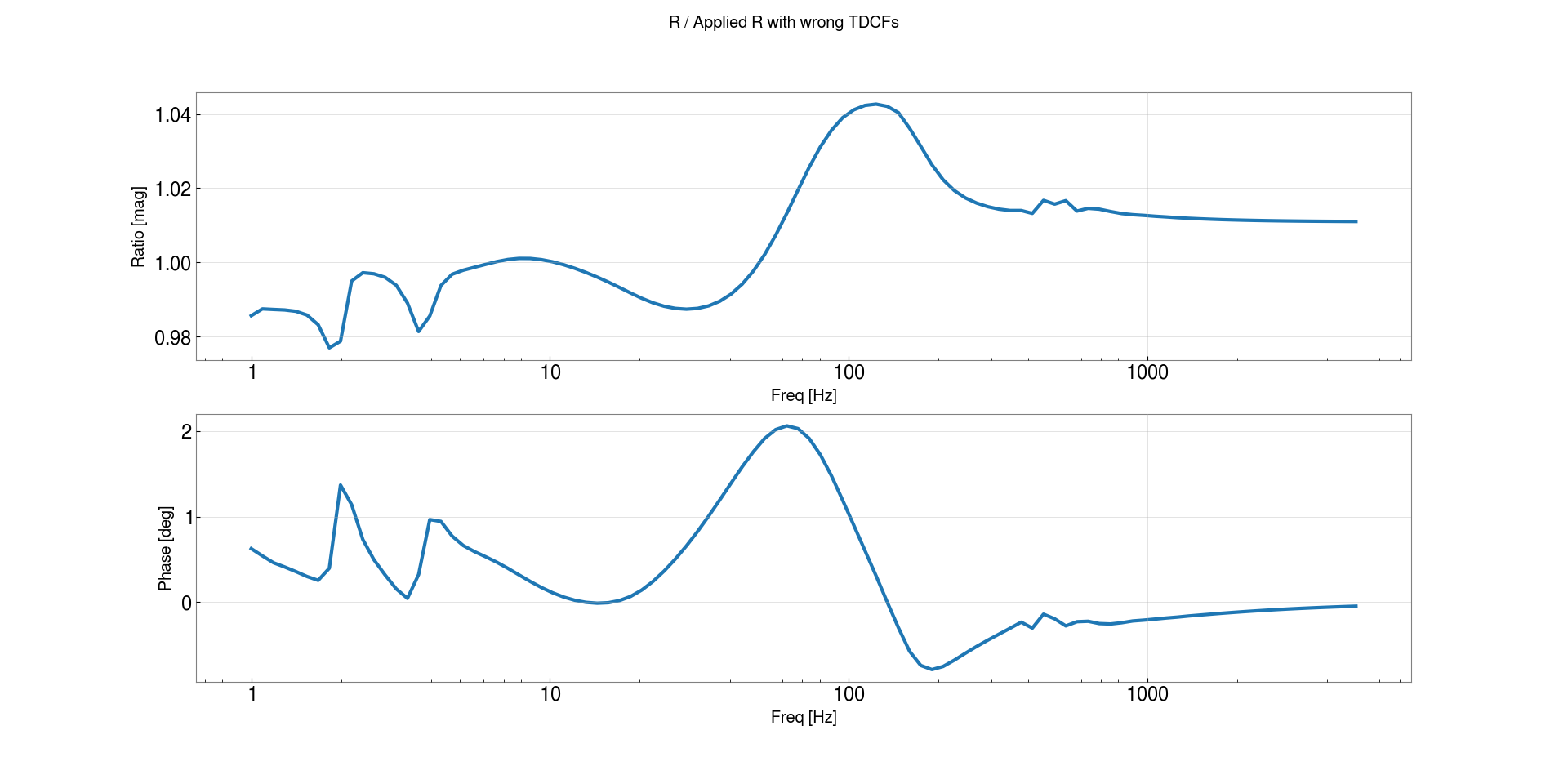
Next we calculate the expected error just from the wrong kappas being
applied in the GDS pipeline due to poor UIM coherence. For this initial look, I choose
GPS time 1374369018 (2023-07-26 01:10 UTC), you can see the LHO summary page here, with
the upper left plot showing the kappa_C discrepancy between GDS and front end.
So just this issue produces the second attachment.
and what he shows in his second attachment, see LHO:72812.
I've made some more clarifying plots to help me better understand Joe's work above after getting a few more details from him and Vlad.

(1) GDS-CALIB_STRAIN is corrected for time dependence, via the relative gain changes, "\kappa," as well as for the new coupled-cavity pole frequency, "f_CC." In order to make a fair comparison between the *measured* response function, GDS-CALIB_STRAIN / DARM_ERR live data stream, and the *modeled* response function, which is static in time, we need to update the response function with the the time dependent correction factors (TDCFs) at the time of the *measured* response function.

How is the *modeled* response function updated for time dependence? Given the new pydarm system, it's actually quite straightforward given a DARM model parameter set, pydarm_H1.ini and good conda environment. Here's a bit of pseudo-code that captures what's happening conceptually:
    # Set up environment
    from gwpy.timeseries import TimeSeriesDict as tsd
    from copy import deepcopy
    import pydarm

    # Instantiate two copies of pydarm DARM loop model
    darmModel_obj = pydarm.darm.DARMModel('pydarm_H1.ini')
    darmModel_wTDCFs_obj = deepcopy(darmModel_obj)

    # Grab time series of TDCFs
    tdcfs = tsd.get(chanList, starttime, endtime, frametype='R',verbose=True)

    kappa_C = tdcfs[chanList[0]].value
    freq_CC = tdcfs[chanList[1]].value
    kappa_U = tdcfs[chanList[2]].value
    kappa_P = tdcfs[chanList[3]].value
    kappa_T = tdcfs[chanList[4]].value

    # Multiply in kappas, replace cavity pole, with a "hot swap" of the relevant parameter in the DARM loop model
    darmModel_wTDCFs_obj.sensing.coupled_cavity_optical_gain *= kappa_C
    darmModel_wTDCFs_obj.sensing.coupled_cavity_pole_frequency = freq_CC
    darmModel_wTDCFs_obj.actuation.xarm.uim_npa *= kappa_U
    darmModel_wTDCFs_obj.actuation.xarm.pum_npa *= kappa_P
    darmModel_wTDCFs_obj.actuation.xarm.tst_npv2 *= kappa_T

    # Extract the response function transfer function on your favorite frequency vector
    R_ref     = darmModel_obj.compute_response_function(freq)
    R_wTDCFs  = darmModel_wTDCFs_obj.compute_response_function(freq)

    # Compare the two response functions to form a "systematic error" transfer function, \eta_R.
    eta_R_wTDCFs_over_ref = R_wTDCFs / R_ref


For all of this study, I started with the reference model parameter set that's relevant for these times in late July 2023 -- the pydarm_H1.ini from the 20230621T211522Z report directory, which I've copied over to a git repo as pydarm_H1_20230621T211522Z.ini.

(2) One layer deeper, some of what Joe's trying to explore in his plots above -- the difference between low-latency, GDS pipeline computed TDCFs and real-time, CALCS pipeline -- because of the issues with the GDS pipeline computation discussed in LHO:72812.

So, in order to facilitate this study, we have to gather TDCFs from both GDS and CALCS pipeline. Here's the channel list for both:
    chanList = ['H1:GRD-ISC_LOCK_STATE_N',

                'H1:CAL-CS_TDEP_KAPPA_C_OUTPUT',
                'H1:CAL-CS_TDEP_F_C_OUTPUT',
                'H1:CAL-CS_TDEP_KAPPA_UIM_REAL_OUTPUT',
                'H1:CAL-CS_TDEP_KAPPA_PUM_REAL_OUTPUT',
                'H1:CAL-CS_TDEP_KAPPA_TST_REAL_OUTPUT',

                'H1:GDS-CALIB_KAPPA_C',
                'H1:GDS-CALIB_F_CC',
                'H1:GDS-CALIB_KAPPA_UIM_REAL',
                'H1:GDS-CALIB_KAPPA_PUM_REAL',
                'H1:GDS-CALIB_KAPPA_TST_REAL']
where the first channel in the list is the state of detector lock acquisition guardian for useful comparison.

(3) Indeed, for *most* of the above aLOG, Joe chooses an example of times when the GDS and CALCS TDCFs are *the most different* -- in his case, 2023-07-26 01:10 UTC (GPS 1374369018) -- when the H1 detector is still thermalizing after power up. They're *different* because the GDS calculation was frozen at the value they were on the day that the calculation was spoiled by a bad MICH FF filter, 2023-08-04 -- and importantly when the detector *was* thermalized.

An important distinction that's not made above, is that the *measured* data in his first plot is from LHO:71787 -- a *different* time, when the detector WAS thermalized, a day later -- 2023-07-27 05:03:20 UTC (GPS 1374469418).

Compare the TDCFs between NOT THERMALIZED time, 2023-07-26 first attachment here with the 2023-07-27 THERMALIZED first attachment I recently added to Vlad's LHO:71787.

One can see in the 2023-07-27 THERMALIZED data, the Frozen GDS and Live CALCS TDCF answers agree quite well. For the NOT THERMALIZED time, 2023-07-26, \kappa_C, f_CC, and \kappa_U are quite different.

(4) So, let's compare the response function ratio, i.e. systematic error transfer function ratio, between the response function updated with GDS TDCFs vs. CALCS TDCFs for the two different times -- thermalizes vs. not thermalized. This will be an expanded version Joe's second attachment:
    - 2nd Attachment here: this exactly replicates Joe's plot, but shows more ratios to better get a feel for what's happening. Using the variables from psuedo code above, I'm plotting
        :: BLUE = eta_R_wTDCFs_CALCS_over_ref = R_wTDCFs_CALCS / R_ref
        :: ORANGE = eta_R_wTDCFs_GDS_over_ref = R_wTDCFs_GDS / R_ref
        :: GREEN = eta_R_wTDCFs_CALCS_over_R_wTDCFs_GDS = R_wTDCFs_CALCS / R_wTDCFs_GDS
    where the GREEN trace is showing what Joe showed -- both as the unlabeled BLUE trace in his second attachment, and the "FE kappa true R / applied bad kappa R" GREEN trace in his third attachment -- the ratio between response functions; one updated with CALCS TDCFs and the other updated with GDS TDCFs, for the NOT THERMALIZED time.

    - 3r Attachment here: this replicates the same traces, but with the TDCFs from Vlad's THERMALIZED time.

For both Joe and my plots, because we think that the CALCS TDCFs are more accurate, and it's tradition to put the more accurate response function in the numerator we show it as such. Comparing the two GREEN traces from my plots, it's much more clear that the difference between GDS and CALCS TDCFs is negligible for THERMALIZED times, and substantial during NOT THERMALIZED times.

(4) Now we bring in the complexity of the missing 3.2 kHz ESD pole. Unlike the "hot swap" of TDCFs in the DARM loop model, it's a lot easier just to create an "offline" copy of the pydarm parameter file, with the ESD poles removed. That parameter file lives in the same git repo location, but called pydarm_H1_20230621T211522Z_no3p2k.ini. So, with that, we just instantiate the model in the same way, but calling the different parameter file:
# Set up environment
    # Instantiate two copies of pydarm DARM loop model
    darmModel_obj = pydarm.darm.DARMModel('pydarm_H1_20230621T211522Z.ini')
    darmModel_no3p2k_obj = pydarm.darm.DARMModel('pydarm_H1_20230621T211522Z_no3p2k.ini')

    # Extract the response function transfer function on your favorite frequency vector
    R_ref = darmModel_obj.compute_response_function(freq)
    R_no3p2k = darmModel_no3p2k_obj.compute_response_function(freq)

    # Compare the two response functions to form a "systematic error" transfer function, \eta_R.
    eta_R_nom_over_no3p2k = R_ref / R_no3p2k

where here, the response function without the 3.2 kHz pole is less accurate, so R_no3p2k goes in the denominator.

Without any TDCF correction, I show this eta_R_nom_over_no3p2k compared against Vlad's fit from LHO:71787 for starters.

(5) Now for the final layer of complexity need to fold in the TDCFs. This is where I think a few more traces and plots are needed comparing the two THERMALIZED vs. NOT times, plus some clear math, in order to explain what's going on. In the end, I make the same conclusion as Joe, that the two effects -- Fixing the Frozen GDS TDCFs and Fixing the 3.2 kHz pole are "separable" to good approximation, but I'm slower than Joe is, and need things laid out more clearly.

So, on the pseudo-code side of things, we need another couple of copies of the darmModel_obj:
    - with and without 3.2 kHz pole
        - with TDCFs from CALCS and GDS,
            - from THERMALIZED (LHO71787) and NOT THERMALIZED (LHO72622) times:

        R_no3p2k_wTDCFs_CCS_LHO71787 = darmModel_no3p2k_wTDCFs_CCS_LHO71787_obj.compute_response_function(freq)
        R_no3p2k_wTDCFs_GDS_LHO71787 = darmModel_no3p2k_wTDCFs_GDS_LHO71787_obj.compute_response_function(freq)
        R_no3p2k_wTDCFs_CCS_LHO72622 = darmModel_no3p2k_wTDCFs_CCS_LHO72622_obj.compute_response_function(freq)
        R_no3p2k_wTDCFs_GDS_LHO72622 = darmModel_no3p2k_wTDCFs_GDS_LHO72622_obj.compute_response_function(freq)


        eta_R_wTDCFS_over_R_wTDCFs_no3p2k_CCS_LHO71787 = R_wTDCFs_CCS_LHO71787 / R_no3p2k_wTDCFs_CCS_LHO71787
        eta_R_wTDCFS_over_R_wTDCFs_no3p2k_GDS_LHO71787 = R_wTDCFs_GDS_LHO71787 / R_no3p2k_wTDCFs_GDS_LHO71787
        eta_R_wTDCFS_over_R_wTDCFs_no3p2k_CCS_LHO72622 = R_wTDCFs_CCS_LHO72622 / R_no3p2k_wTDCFs_CCS_LHO72622
        eta_R_wTDCFS_over_R_wTDCFs_no3p2k_GDS_LHO72622 = R_wTDCFs_GDS_LHO72622 / R_no3p2k_wTDCFs_GDS_LHO72622


Note, critically, that these ratios of with and without the 3.2 kHz pole -- both updated with the same TDCFs -- is NOT THE SAME THING as just the ratio of models updated with GDS vs CALCS TDCFs, even though it might look like the "reference" and "no 3.2 kHz pole" might cancel "on paper," if one naively thinks that the operation is separable

    [[ ( R_wTDCFs_CCS / R_ref )*( R_ref / R_no3p2k ) ]] / [[ ( R_wTDCFs_GDS / R_ref )*(R_ref / R_no3p2k) ]] #NAIVE
    which one might naively cancel terms to get down to
    [[ ( R_wTDCFs_CCS / R_ref )*( R_ref / R_no3p2k ) ]] / [[ ( R_wTDCFs_GDS / R_ref )*(R_ref / R_no3p2k) ]]  #NAIVE
    [[ ( R_wTDCFs_CCS ]] / [[ R_wTDCFs_GDS ]] #NAIVE


So, let's look at the answer now, with all this context.
    - NOT THERMALIZED This is a replica of what Joe shows in the third attachment for the 2023-07-26 time:
        :: BLUE -- the systematic error incurred from excluding the 3.2 kHz pole on the reference response function without any updates to TDCFs (eta_R_nom_over_no3p2k)
        :: ORANGE -- the systematic error incurred from excluding the 3.2 kHz pole on the CALCS-TDCF-updated, modeled response function (eta_R_wTDCFS_over_R_wTDCFs_no3p2k_CCS_LHO72622, Joe's "FE kappa true R /applied R (no pole))
        :: GREEN -- the systematic error incurred from excluding the 3.2 kHz pole on the GDS-TDCF-updated, modeled response function (eta_R_wTDCFS_over_R_wTDCFs_no3p2k_GDS_LHO72622, Joe's "GDS kappa true R / applied (no pole)")
        :: RED -- Compared against Vlad's *fit* the ratio of CALCS-TDCF-updated, modeled response function to (GDS-CALIB_STRAIN / DARM_ERR) measured response function

    Here, because the GDS TDCFs are different than the CALCS TDCFs, you actually see a non-negligible difference between ORANGE and GREEN.

    - THERMALIZED:
        (Same legend, but the TIME and TDCFs are different)

    Here, because the GDS and CALCS TDCFs are the same-ish, you can't see that much of a difference between the two.

    Also, note, that even when we're using the same THERMALIZED time and corresponding TDCFs to be self-consistent with Vlad's fit of the measured response function, they still don't agree perfectly. So, there's likely still yet more systematic error going in the thermalized time.

(6) Finally, I wanted to explicitly show the consequences of "just" correcting for GDS and from "just" correcting the missing 3.2 kHz pole to be able to better *quantify* the statement that "the difference is pretty small compared to typical calibration uncertainties," as well as showing the difference between "just" the ratio response functions updated with the different TDCFs (the incorrect model), against the "full" models.

    I show this in
    - NOT THERMALIZED, and
    - THERMALIZED

For both of these plots, I show
    :: GREEN -- the corrective transfer function we would be applying if we only update the Frozen GDS TDCFs to Live CALCS TDCFs, compared with
    :: BLUE -- the ratio of corrective transfer functions,
         >> the "best we could do," updating the response with Live TDCFs from CALCS and fixing the missing 3.2 kHz pole against
         >> only fixing the missing 3.2 kHz pole
    :: ORANGE -- the ratio of corrective transfer functions
         >> the "best we could do," updating the response with Live TDCFs from CALCS and fixing the missing 3.2 kHz pole against
         >> the "second best thing to do" which is leave the Frozen TDCFs alone and correct for the missing 3.2 kHz pole

     Even for the NOT THERMALIZED time, the BLUE never exceeds 1.002 / 0.1 deg in magnitude / phase, and it's small compared to the "TDCF only" the simple correction of Frozen GDS TDCFs to Live CALCS TDCFs, shown in GREEN .  This helps quantify why Joe thinks we can separately apply the two corrections to the systematic error budget, because GREEN is much larger than BLUE.

    For the THERMALIZED time, in BLUE, that ratio of full models is even less, and also as expected the ratio of simple TDCF update models is also small.


%%%%%%%%%%
The code that produced this aLOG is create_no3p2kHz_syserror.py as of git hash 3d8dd5df.
Non-image files attached to this comment

Following up on this study just one step further, as I begin to actually correct data curing the time period where both of these systematic errors are in play -- the frozen GDS TDCFs and the missing 3.2 kHZ pole...

I craved one more set of plots to convey "Fixing the Frozen GDS TDCFs and Fixing the 3.2 kHz pole are "separable" to good approximation" showing the actual corrections one would apply in the different cases:
    :: BLUE = eta_R_nom_over_no3p2k = R_ref / R_no3p2k >> The systematic error created by the missing 3.2 kHz pole in the ESD model alone
    :: ORANGE = eta_R_wTDCFs_CALCS_over_R_wTDCFs_GDS = R_wTDCFs_CALCS / R_wTDCFs_GDS >> the systematic error created by the frozen GDS TDCFs alone
    :: GREEN = eta_R_nom_over_no3p2k * eta_R_wTDCFs_CALCS_over_R_wTDCFs_GDS = the product of the two >> the approximation
    :: RED = a previously unshown eta that we'd actually apply to the data that had both = R_ref (updated with CALCS TDCFS) / R_no3p2k (updated with GDS TDCFs) the right thing

As above, it's important to look at both a thermalized case as well as a non-thermalized case., so I attach those two,
    NOT THERMALIZED, and
    THERMALIZED.

The conclusions are the same as above:
    - Joe is again right that the difference between the approximation (GREEN) and the right thing (RED) is small, even for the NOT THERMALIZED time
But I think this version of the plots / traces better shows the breakdown of which effect is contribution where on top of the approximation vs. "the right thing," and "the right thing" was never explicitly shown. All the traces in my expanded aLOG, LHO:72879, had the reference model (or no 3.2 kHz pole models) updated either both CALCS TDCFs or both GDS TDCFs in the numerator and denominator, rather than "the right thing" where you have CALCS TDCFs in the numerator and GDS TDCFs in the denominator).

%%%%%%%%%%%%%%%%%%%%%%%%%%%%%%%%%%%%%
To create these extra plots, I added a few lines of "calculation" code and another 40-ish lines of plotting code to create_no3p2kHz_syserror.py. I've now updated in within the git repo, so it and the repo now have git hash 1c0a4126.
Non-image files attached to this comment